Optimization

Thread: how feasible two-asset weights change with budget, leverage and long-only bounds, and how the objective and KKT conditions check a solution.

Begin with constructed one-year inputs. Assets 1 and 2 have expected total returns $(0.05,0.08)$ and covariance matrix

Let $w_1=x$ and $w_2=1-x$. Budget $w_1+w_2=1$ and long-only lower bounds $w_1,w_2\geq0$ imply $x\in[0,1]$. Compare feasible points using $J(w)=\tfrac12\lambda w^\top\Sigma w-\mu^\top w$ with $\lambda=1$:

All three points satisfy budget and long-only constraints. They indicate direction, without proving optimality over the continuous interval. $w$ contains dimensionless weights, $\mu$ expected total returns over the same annual holding period, and $\Sigma$ squared-decimal-return covariance. Risk coefficient $\lambda$ has inverse-decimal-return units, making both objective terms annual decimal returns. Return from these feasible points to the full model to derive the optimum.

Prerequisites: calculus in Chapter 4, linear algebra in Chapter 5 and regression in Chapter 8. You will prove quadratic convexity, formulate least squares, LP and mean–variance QP, distinguish necessary from sufficient KKT conditions, interpret local dual shadow prices, and check CVXPY statuses and constraint residuals.

1. Learning objectives

Separate four layers. Variables identify choices, dimensions and units. The objective compresses return, risk or fitting error to a scalar. The feasible set describes budget, long-only and capacity limits. Evidence consists of solver status, primal feasibility, dual quantities and residuals supporting the conclusion.

By the end, you should be able to:

1. Distinguish objective functions, decision variables, constraints, feasible points and optimal points.
2. Prove set/function convexity by definition, second derivatives or Hessians, recognizing positive definiteness as one sufficient route to strict convexity.
3. Formulate least squares as a convex quadratic program (QP) and state rank or tangent-space conditions for uniqueness.
4. Write linear programs (LPs) and mean–variance QPs, tracking input, output, objective and dual units.
5. Derive weak duality, complementary slackness, Karush–Kuhn–Tucker (KKT) conditions and right-hand-side shadow prices from the Lagrangian.
6. Explain Slater’s role in strong duality and KKT’s different logical status in nonconvex and convex problems.
7. Inspect CVXPY solver status, feasibility residuals and KKT diagnostics, including optimal_inaccurate, infeasibility, unboundedness and the limits of handling slightly negative covariance eigenvalues.

Numerical checks concern fixed constructions: mean–variance weights $[5/11,6/11]$ and minimum-variance weights $[8/11,3/11]$; a $0.4$ cap on each of two assets is infeasible. At risk aversion $0.2$ the optimum is boundary $[0,1]$ with first long-only-bound dual $0.014$. The constructed production LP chooses 40 A batches and 20 B batches per day for 160 thousand euros of daily contribution. These are teaching numbers, not market estimates or backtest returns.

2. Why a quant needs optimization

Statistics asks what an unknown quantity might be given observations. Optimization asks which portfolio, order or resource allocation to choose given estimates and feasible choices. They connect without replacing one another. Mean–variance optimization uses expected returns $\mu$ and covariance $\Sigma$. A solver finds weights for those inputs, without verifying their estimation accuracy or that future trades can execute at the mathematically optimal weights.

Without explicit objectives, code can confuse volatility, variance, absolute loss and drawdown. Without feasible constraints, it can output impossible short positions, excessive gross exposure or overused resources. Without status and independent residual checks, a floating-point vector in x.value can be mistaken for a validated strategy. Researchers must define the complete problem before asking a numerical solver to solve it.

Three structures connect the chapter. Least squares expresses Chapter 8’s squared-error objective as an unconstrained convex QP. LP distributes scarce resources through a linear objective on a polyhedral feasible set. Mean–variance QP chooses between expected return and risk. Each needs an objective, feasible set and optimality check, but their units, solution methods and economic interpretations differ.

3. Intuition: draw feasible choices before seeking improvement

Put asset 1’s weight on a horizontal axis and asset 2’s on a vertical axis. Full investment gives line $w_1+w_2=1$; nonnegative weights restrict it to the segment from $(0,1)$ to $(1,0)$. Each point is an allowed portfolio. The mean–variance objective becomes a quadratic curve along that segment. Optimize over the segment, rather than seeking an arbitrary zero gradient in the plane.

A convex set contains the segment between any two points. With a convex objective on that set, a feasible local optimum is global; there is no inferior local valley. Strict convexity permits at most one optimum. Algorithms still iterate and use floating-point approximations, but the mathematical structure excludes separated local valleys.

LP level sets are parallel lines, and a linear objective commonly improves toward a polygon vertex. QP contours are ellipses or degenerate ellipses; optima may be interior or constrained to a boundary. A boundary optimum generally has nonzero full-space gradient. Ask instead whether any feasible direction can reduce the objective; constrained optimality and KKT express this.

Nonconvex objectives can have multiple local extrema; nonconvex constraints can disconnect the feasible set. A convex solver does not turn an incorrectly chosen objective into a valid research question.

4. Mathematical foundations: dimensions, units and feasible choices

Dimensional checks reveal modeling errors early. For $x$ in batches/day, $Ax\leq b$ needs $A_{ij}$ in resource-hours/batch and $b_i$ in resource-hours/day, so $Ax$ and $b$ match. If $c_j$ is thousand euros/batch, $c^\top x$ is thousand euros/day. Portfolio weights $w\in\mathbb{R}^n$ are dimensionless, expected return $\mu_i$ is a decimal over the holding period, and $\Sigma_{ij}$ is same-period covariance in squared-decimal-return units. $w^\top\Sigma w$ is portfolio-return variance.

The example’s holding period is one year: $0.05$ means expected simple return $5\%$ over that year, and covariance concerns annual decimal returns. Neither input is rescaled independently. Risk aversion $\lambda$ has inverse-decimal-return units, making $\lambda w^\top\Sigma w$ and $\mu^\top w$ both annual decimal returns. Weights summing to 1 is a budget identity, not an observed return or trade time.

Distinguish feasibility, boundedness, attainment and numerical verification. Feasibility requires at least one allowed point; boundedness a finite best objective value; attainment a feasible point realizing that value; numerical verification sufficient precision and compliance with model contracts in the returned floating-point result. A problem can be infeasible, or feasible but unbounded. optimal_inaccurate reports a lower-precision candidate, distinct from optimal. Even optimal returns floating-point values requiring residual and application-precision checks. Printing weights does not establish all four layers.

5. Definitions: convex problems, LP, QP and feasibility

A set $C$ is convex when all $x,y\in C$ and $\theta\in[0,1]$ satisfy $\theta x+(1-\theta)y\in C$. A convex combination uses nonnegative weights summing to 1; fully invested long-only portfolios form a convex simplex. Half-spaces $a^\top x\leq b$, affine-equality solution sets $Ax=b$ and their intersections are convex. A convex function satisfies

Geometrically, the graph lies below its chords. Strict inequality for distinct $x,y$ and $0<\theta<1$ defines strict convexity. Convex optimization minimizes a convex objective on a convex feasible set; equivalently it can maximize a concave objective. A local optimum is global. Strict convexity allows at most one optimum on that set, without guaranteeing its existence.

For the quadratic function

take symmetric $P\in\mathbb{R}^{n\times n}$, with $c\in\mathbb{R}^n$, $x\in\mathbb{R}^n$ and $r\in\mathbb{R}$. Its Hessian is $P$. If $P\succeq0$, every direction $d$ has curvature $d^\top P d\geq0$ and $q$ is convex. If $P\succ0$, every nonzero direction has positive curvature and $q$ is strictly convex. Positive definiteness is sufficient and also necessary for a quadratic to be strictly convex on the full space. On a budget hyperplane, even singular $P$ can give strict convexity when curvature is positive in every nonzero feasible direction.

A linear program (LP) has a linear objective and affine constraints, for example

With $x\in\mathbb{R}^n$ and $m$ resource constraints, dimensions are $A\in\mathbb{R}^{m\times n}$, $b\in\mathbb{R}^m$ and $c\in\mathbb{R}^n$. Linear objectives are both convex and concave; the feasible region is polyhedral. LP is the QP special case $P=0$.

General quadratic programs can be nonconvex. This chapter considers convex QP only: positive-semidefinite quadratic objective matrices with linear equalities/inequalities:

Here $G\in\mathbb{R}^{m\times n}$, $h\in\mathbb{R}^m$, $A\in\mathbb{R}^{p\times n}$ and $b\in\mathbb{R}^p$. Finitely many linear constraints in finite dimensions define a closed polyhedron. A coercive objective on the feasible set, or a continuous objective on a compact feasible set, are two common sufficient existence conditions, not necessary ones. A convex QP on a closed polyhedron also attains a finite optimum; details lie beyond this chapter. Convexity alone does not guarantee existence or convergence within default solver precision.

CVXPY uses disciplined convex programming (DCP) rules: minimize expressions certified convex, maximize expressions certified concave, and combine affine equalities with correctly oriented convex/concave inequalities. Passing DCP verifies expression rules, not units, economic suitability or estimation accuracy. Failing DCP need not prove mathematical nonconvexity; the expression may lie outside its rules and require an equivalent reformulation.

6. Derivations: from curvature to KKT and duality

6.1 Why a PSD Hessian makes a quadratic convex

Let $P=P^\top\succeq0$ and choose points $x,y$ and $\theta\in[0,1]$. On expansion, linear term $c^\top x$ and constant $r$ cancel in the convex-combination difference:

Positive semidefiniteness gives the last inequality, hence convexity. Conversely, if a direction $d$ has $d^\top P d<0$, curvature along $x+td$ is negative, so the quadratic is not globally convex. Symmetrizing does not generally repair invalid covariance. Theoretical covariance is symmetric PSD; small numerical asymmetry may be averaged within declared tolerances, but material asymmetry or negative eigenvalues require an audit of data and estimation.

6.2 Why least squares is a QP

Let design $A\in\mathbb{R}^{m\times n}$, observations $y\in\mathbb{R}^m$ and chosen coefficients $\beta\in\mathbb{R}^n$ define least squares:

Expanding the square gives

$A^\top A$ is PSD because every $z$ satisfies $z^\top A^\top A z=\|Az\|_2^2\geq0$. The residual sum of squares is therefore convex quadratic. Differentiating in $\beta$ gives $2A^\top(A\beta-y)$ and the normal equations $A^\top A\beta=A^\top y$. Full column rank of $A$ gives $A^\top A\succ0$ and unique coefficients. Otherwise fitted values remain unique but coefficients do not. Explicit inversion $(A^\top A)^{-1}$ amplifies ill-conditioning; prefer numpy.linalg.lstsq, QR/SVD or a reliable least-squares solver.

This does not repeat Chapter 8’s inference. Optimization finds coefficients minimizing squared error; it supplies no standard errors, tests, error diagnostics or information-timing evidence for prediction.

6.3 Lagrangian, weak duality and Slater’s condition

In Section 4’s general minimization problem, attach nonnegative multiplier $\lambda_i\geq0$ to inequality $f_i(x)\leq0$ and unrestricted multiplier $\nu_j\in\mathbb{R}$ to each equality. The Lagrangian is

For feasible $x$, $\lambda_i f_i(x)\leq0$ and equality terms vanish, giving $L(x,\lambda,\nu)\leq f_0(x)$. Taking the infimum over $x$ gives dual function $g(\lambda,\nu)=\inf_x L(x,\lambda,\nu)$, a lower bound on every feasible primal objective. Maximizing it yields the Lagrangian dual problem. Dual optimum $d^\star$ never exceeds primal optimum $p^\star$: $d^\star\leq p^\star$. This weak duality also holds for nonconvex problems.

Equality of optimal values is strong duality. For convex problems, Slater is a sufficient constraint qualification; with finite primal optimum, it also ensures dual attainment. It is not necessary. Standard Slater requires a point in the relative interior of the common domain satisfying affine equalities and strictly satisfying every convex inequality. The refined version allows non-strict affine inequalities but still requires strict nonaffine convex inequalities. With only affine inequalities, as in these QPs, a feasible point in the domain’s relative interior suffices without strict inequality; these quadratic domains are all of $\mathbb{R}^n$. Failure of this sufficient condition does not establish failure of strong duality.

6.4 When KKT conditions are necessary or sufficient

For differentiable problems, Karush–Kuhn–Tucker (KKT) conditions consist of four groups:

Stationarity balances objective gradients with constraint effects. Complementary slackness makes inactive-inequality multipliers zero, and positive multipliers require active constraints. An active constraint can still have zero multiplier; a boundary does not necessarily have a positive shadow price.

6.5 Shadow prices and perturbations

For resource bounds $Ax\leq b$, dual multipliers $\lambda^\star\geq0$ attach to resource constraints. Near a regular LP basis, a small relaxation $\Delta b_i$ of resource bound $b_i$ for row $i$ changes maximum contribution by approximately $\lambda_i^\star\Delta b_i$. Multipliers have objective-units/resource-units, allowing comparison of scarce capacity with added contribution. This first-order interpretation needs a stable active structure; crossing vertices, changing active sets or meeting a nondifferentiable value function prevents distant linear extrapolation.

For minimization with perturbation $f_i(x)\leq u_i$ and a differentiable value function, $\partial p^\star/\partial u_i=-\lambda_i^\star$. Relaxing upper bound $u_i$ generally reduces minimum cost, with the sign set by this inequality orientation. In the usual maximization LP $Ax\leq b$, resource-value derivatives are nonnegative $\lambda_i^\star$. Specify objective direction and right-hand-side perturbation before interpreting a sign.

7. Financial interpretation: optimizing estimated models, not future returns

Mean–variance portfolios combine weights $w\in\mathbb{R}^n$, same-horizon expected returns $\mu\in\mathbb{R}^n$ and covariance $\Sigma\in\mathbb{R}^{n\times n}$ into a QP:

The first term penalizes variance and the second rewards expected return. The negative sign makes maximizing return equivalent to minimizing negative return here. With annual decimal simple returns, $w$ is dimensionless, $\mu^\top w$ annual expected decimal return, $w^\top\Sigma w$ annual squared-decimal-return variance, and $\lambda$ inverse-decimal-return risk aversion. Both objective terms then share units.

Increasing $\lambda$ emphasizes variance over estimated mean; decreasing $\lambda$ emphasizes return and can push weights toward higher estimated means or constraint boundaries. Weights are model decisions conditional on estimates, not intervals for future returns. Mean estimates are noisy; covariance perturbations can change weights. Assess estimation windows, shrinkage, caps, turnover, costs, borrowing and risk budgets.

Maximum Sharpe uses expected excess returns. Let $r_f$ be the risk-free benchmark for the same holding period and currency and define $\mu^{ex}=\mathbb{E}[R]-r_f\mathbf{1}$. Subtract same-period $r_f$ from total-return inputs; if no risk-free benchmark is modeled, explicitly assume $r_f=0$. Do not combine monthly excess returns with annual risk-free rates. The objective is

This fractional objective cannot be used directly as an ordinary QP objective under DCP. Let $C$ be the convex set defined by budget, long-only and optional linear weight caps. First confirm that the finite-ratio candidate domain

is nonempty. $\Sigma\succeq0$ alone does not ensure that. An empty original domain has no finite positive-Sharpe candidates of the type discussed here.

Budget $\mathbf1^\top w=1$ is not itself invariant to scaling. For $w\in D_w$, set $y=w/((\mu^{ex})^\top w)$. Then $y\ge0$, $(\mu^{ex})^\top y=1$ and

The reverse direction must preserve positive variance too: given $y\ge0$, $(\mu^{ex})^\top y=1$ and $y^\top\Sigma y>0$, set $t=\mathbf1^\top y>0$ and $w=y/t$, obtaining $(\mu^{ex})^\top w=1/t>0$ and $w^\top\Sigma w=y^\top\Sigma y/t^2>0$. Weight cap $w_i\le c_i$ becomes $y_i\le c_i\mathbf1^\top y$ in both directions. Denote the closed polyhedron without the positive-variance condition by $\overline D_y$ and the strict corresponding domain by $D_y=\{y\in\overline D_y:y^\top\Sigma y>0\}$. The bidirectional mapping holds only between $D_w$ and $D_y$ and preserves Sharpe ordering:

The solvable closed convex QP minimizes $q(y)=y^\top\Sigma y$ on $\overline D_y$; distinguish it from the strict domain. Assume its minimum is attained. If $q^\star>0$, its optimizer lies in $D_y$ and transforms back to finite maximum Sharpe $1/\sqrt{q^\star}$. If $q^\star=0$, the zero-variance optimizer lies outside $D_y$ and cannot be reported as a finite-ratio optimum. Confirmed $D_w\ne\varnothing$ provides a positive-variance feasible point. Under the present convex budget/long-only/linear-cap structure, mixing it with the zero-variance point generates finite ratios tending to infinity. Section 18 proves supremum $+\infty$; the zero-variance point’s own ratio is undefined. Do not draw this conclusion for an empty original domain.

$\Sigma\succ0$ is a simple sufficient condition for every nonzero transformed vector to have positive variance, not a necessary condition for a finite optimum. Adding strict $q(y)>0$ does not make an ordinary convex QP: a convex quadratic’s strict superlevel set is generally nonconvex. Prove that transformations and mixtures preserve any costs, fixed amounts or other complex restrictions separately.

8. Numerical Example

8.2 Checking least squares and a resource LP by hand

Construct features $x=(0,1,2,3)$ and response $y=(1,2,4,5)$ in arbitrary teaching units, not market returns. Intercept design $A$ has rows $(1,x_i)$, giving

Normal equations are $4\beta_0+6\beta_1=12$ and $6\beta_0+14\beta_1=25$. Subtract 1.5 times the first from the second to obtain $5\beta_1=7$, hence slope $\beta_1=1.4$ and intercept $\beta_0=0.9$. Fits $(0.9,2.3,3.7,5.1)$ and residuals $(0.1,-0.3,0.3,-0.1)$ give squared loss $0.2$. Full column rank of $A$ makes the loss strictly convex and these coefficients uniquely optimal, without establishing statistical significance.

9. Python Implementation

Default entry in the accepted reader package

From the accepted I3 reader-package root, create the isolated environment described in its README, then run:

.venv/bin/python run_notebook.py notebooks/ch09_optimization.ipynb

The notebook calls the packaged shared implementation. It reads no omitted French data and downloads none by default. Every execution and its figures go into a unique UUID runs directory, whose actual location is printed. Old production tests and historical commands below belong to the course working project; the default reader route uses the package-root notebook and its assertions. Optional historical data follows the reader’s data contract; this batch did not rerun it.

I3 also includes code/ch09_optimization.py, but the default reader entry remains the notebook above.

Historical course-root route

Previously validated core functions are in optimization_tools.py, with standalone example ch09_optimization.py. From the course-project root, run:

.venv/bin/python code/ch09_optimization.py

The recorded script used CVXPY 1.9.3 with installed solvers CLARABEL, SCS, SCIPY, HIGHS and OSQP. OSQP returned optimal for the convex QP, while the LP used CLARABEL. Defaults can differ between environments. Report actual problem.solver_stats.solver_name; do not assume every installation has the same solver.

Run this minimal portfolio example independently from that project root:

import sys
sys.path.insert(0, "src")
import numpy as np
from quant_course.optimization_tools import solve_mean_variance

mu = np.array([0.05, 0.08])
sigma = np.array([[0.04, 0.01], [0.01, 0.09]])
result = solve_mean_variance(mu, sigma, risk_aversion=1.0, solver="OSQP")
minimum_variance = solve_mean_variance([0.0, 0.0], sigma, solver="OSQP")
print(result.solver_status, result.solver_name, result.weights)
print(result.expected_return, result.variance, result.objective)
print("primal residuals", result.budget_residual, result.nonnegativity_violation)
print("KKT diagnostics", result.stationarity_residual, result.complementarity_residual)
print("min-variance", minimum_variance.weights, minimum_variance.variance)
assert np.allclose(result.weights, [5 / 11, 6 / 11], atol=1e-7)

The wrapper requires a finite real expected-return vector, matching finite approximately symmetric PSD covariance, positive risk aversion and feasibility tolerance, and optional weight cap in $(0,1]$. Invalid dimensions, finite values, symmetry or semidefiniteness raise errors. Eigenvalue tolerance is $10^{-10}\max_i|d_i|$, where $d_i$ are eigenvalues. Values below negative tolerance are rejected; slightly negative values within tolerance are clipped to zero and the matrix reconstructed. This permits only negative curvature small relative to spectral scale, without proving rounding caused it. A zero matrix has zero spectral scale and tolerance; no absolute tolerance floor is added. Symmetry is also checked relative to the largest absolute matrix entry. This is not a general remedy for economic estimation errors; the return object has no separate clipping flag.

After modeling, check problem.is_dcp(), solve and inspect status:

• optimal: proceed to independent feasibility checks.
• optimal_inaccurate: reject as a passed result.

The wrapper independently recomputes budget, long-only and upper-bound violations, raising an error if their maximum exceeds default $10^{-6}$. It also returns stationarity and complementary-slackness residuals and checks they are finite. It sets no acceptance threshold for these two KKT residuals and checks neither dual signs, dual gap nor a convergence-precision certificate. They are diagnostics, not proof that every solve passed a complete KKT certificate. The objective uses the covariance after eigenvalue validation; clipping slightly negative eigenvalues makes diagnostics refer to that modified model.

Financial inputs use one-year horizons. The script contains no real prices, release dates, signals, executions or realized holding intervals. There are no available_at, signal_time or trade_time fields to audit, and no period-start signal predicts subsequent realized returns. Real research requires estimation-window data available before signal generation and timing $\text{signal\_time}<\text{trade\_time}\leq\text{return interval start}$. Holding-period length must match $\mu$ and $\Sigma$ units.

10. Visualization

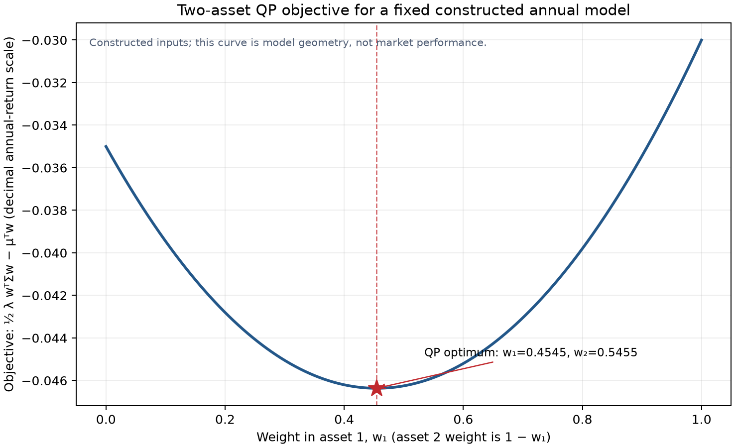
The script generated the following objective curve:

The horizontal axis is asset 1 weight $w_1\in[0,1]$; asset 2 automatically has $1-w_1$. The vertical axis is annual-decimal-return objective $\frac12\lambda w^\top\Sigma w-\mu^\top w$. Fixed constructed inputs generate the curve; the red star and dashed line mark interior weights $w_1=5/11$ and $w_2=6/11$. Upward curvature reflects a positive second derivative, with larger objective values toward either endpoint.

The figure describes model geometry, not asset-return history, an empirical efficient frontier or performance. Minimum $-0.04636$ is an objective value containing a variance penalty, not expected return, annual Sharpe or net portfolio return. The plotted objective agrees with script output.

11. Real Market Example

This chapter reads no real asset prices or returns and reports no empirical portfolios, optimal market weights or out-of-sample performance. Two-asset $\mu$ and $\Sigma$, LP profits/capacity and the four least-squares points are constructions. The contribution is a method for turning estimates into decisions and checking solutions, not empirical market evidence.

A real study needs a fixed security universe and delisting treatment; total versus price returns, risk-free series, currency, adjustments and forecast frequency; and saved versions, download time, sample windows and hashes. Estimate means, covariance and features only from point-in-time available information, using training alone for tuning and risk budgets. Validate signals through order submission/execution and post-trade holding returns, comparing simple benchmarks, turnover, costs, slippage, capacity and robust parameter ranges.

12. Common Mistakes

Calling maximized convex risk a DCP problem. For PSD $\Sigma$, $w^\top\Sigma w$ is convex. DCP permits minimizing, not maximizing, a convex expression. Define the intended minimized risk–return objective and verify constraints.

import cvxpy as cp
import numpy as np

mu = np.array([0.05, 0.08])
sigma = np.array([[0.04, 0.01], [0.01, 0.09]])
w = cp.Variable(2)
constraints = [cp.sum(w) == 1, w >= 0]
wrong = cp.Problem(cp.Maximize(cp.quad_form(w, sigma)), constraints)
print("wrong problem follows DCP:", wrong.is_dcp())
try:
    wrong.solve(solver="OSQP")
except cp.error.DCPError as error:
    print(type(error).__name__)
correct = cp.Problem(
    cp.Minimize(0.5 * cp.quad_form(w, sigma) - mu @ w), constraints
)
print("correct problem follows DCP:", correct.is_dcp())
correct.solve(solver="OSQP")
print(correct.status, w.value)

The incorrect model fails DCP with False and raises DCPError; the corrected model gives True and optimal. If the research objective truly calls for maximum risk, its risk definition may be reversed. Changing maximization to minimization is a modeling decision requiring review of the hypothesis, not merely a syntax correction.

Mixing return and covariance horizons. Annual expected returns with unscaled monthly covariance distort the risk term. Unify holding period and return scale first. Aggregating monthly independent increments to a year requires independence or appropriate weak-correlation assumptions for covariance scaling; “multiply by 12” does not verify frequency structure. One-year inputs here are constructions, not a data-annualization procedure.

Passing a low-precision status as normal success. optimal_inaccurate supplies a low-precision candidate; infeasible_inaccurate limits the precision of an infeasibility conclusion. Nonempty value alone can hide boundary violations. The following checks show conservative API behavior: impossible caps raise OptimizationError preserving status, while a materially non-PSD covariance fails before modeling.

import sys
sys.path.insert(0, "src")
from quant_course.optimization_tools import OptimizationError, solve_mean_variance

mu = [0.05, 0.08]
sigma = [[0.04, 0.01], [0.01, 0.09]]
try:
    solve_mean_variance(mu, sigma, max_weight=0.4, solver="CLARABEL")
except OptimizationError as error:
    print("cap result:", error.solver_status)
try:
    solve_mean_variance(mu, [[1.0, 2.0], [2.0, 1.0]], solver="CLARABEL")
except ValueError as error:
    print("covariance rejected:", str(error))
valid = solve_mean_variance(mu, sigma, solver="CLARABEL")
print(valid.solver_status, "budget residual", valid.budget_residual)
print("reported KKT diagnostics", valid.stationarity_residual, valid.complementarity_residual)

Recorded outputs show infeasible, rejection of the non-PSD matrix, and optimal for the valid QP. If numerically unstable, report status and inspect scaling, conditioning, PSD, primal constraints and solver logs; reformulate or compare other installed solvers as needed. Do not silently treat candidate weights as usable.

Turning a nonzero dual into a large-return guarantee. Interpret it under the current objective, constraint direction, active set and local perturbation. Changing a right-hand side may change vertices or units, preventing distant extrapolation. Track CVXPY inequality orientation and Lagrangian signs: w >= 0 has a lower-bound multiplier entering stationarity with a minus sign.

Rejecting a boundary solution because the full-space gradient is nonzero. Unconstrained interior optima have zero gradients; boundaries restrict feasible directions. KKT balances objective gradients with budget and bound gradients. At risk aversion $\lambda=0.2$ in the two-asset example, the original gradient is nonzero but the inward budget-line derivative is positive, so the boundary solution is optimal.

Sending every maximum-Sharpe problem directly to QP. The fractional objective depends on $\sqrt{w^\top\Sigma w}$; direct Maximize is not ordinary QP/DCP. Restrict to positive excess return and positive variance, prove bidirectional feasibility, normalize budget on transforming back, and translate fixed weight caps to homogeneous linear constraints.

13. Quant Research Application

Start with the research question: portfolio choice, execution planning or analysis of a fitting objective? Fix horizon and units, list decisions, objective, equalities, bounds and inviolable risk budgets. Portfolio inputs need security identities, return definition, currency, risk-free return, adjustments, delistings, covariance windows and mean-estimation methods. Audit available_at, versions and signal times, then establish convexity and feasibility before creating CVXPY expressions.

Do not transfer $w^\star$ directly into a performance report. Check status, returned variables and actual solver. Independently recompute $\mathbf{1}^\top w-1$, minimum/maximum weights, budget and risk residuals; inspect multipliers, active constraints, stationarity and complementarity. Stress estimates: can small mean perturbations, covariance shrinkage, asset exclusions or risk-aversion changes reverse the portfolio? Local shadow prices do not replace sensitivity analysis.

At each real backtest period, estimate $\mu$ and $\Sigma$ only from then-available historical observations. Generate signal_time before feasible trade_time, then map weights to an explicit post-trade return interval. Align holding period, estimation frequency, risk matrix and cost timing. Optimization must not use later revisions, future prices or holdout targets. Record benchmarks, turnover, fees, slippage, borrowing, capacity and rebalancing. Prespecify disconfirmation, such as weights flipping under reasonable mean estimates, excess out-of-sample risk, failure after costs or contradictory constraints/execution rules.

The script provides no point-in-time data, signals, trades or holding-period performance. It demonstrates objectives, convexity, solver outputs and structural checks, without empirical strategy effects.

Further research boundaries appear in Chapter 20: modern portfolio theory and Chapter 21: practical portfolio construction. Chapter 20 distinguishes population from estimated moments and treats plug-in frontiers as in-sample objects. Chapter 21 addresses mean/covariance error, real holdings constraints, turnover/cost ledgers and out-of-sample evaluation. A constructed optimum alone establishes neither improved real return nor executability.

14. Chapter Summary

Optimization defines an objective with its feasible region. Convex objectives on convex sets have globally optimal local optima; PSD Hessians produce typical convex QPs. Least-squares Gram matrix $A^\top A$ is PSD; LP uses linear resource bounds; mean–variance QP combines convex risk with expected return.

Lagrange multipliers incorporate constraints and relate primal and dual problems. Weak duality always provides a bound. Convexity with qualifications such as Slater can establish strong duality. Feasible KKT conditions suffice in convex problems; in general nonconvex problems they commonly provide necessary stationarity under regularity. Dual sensitivity remains local, with signs, units and perturbation directions set by constraint conventions.

Solver status is computational evidence, not economic evidence. Report solver, status, objective, primal residuals, KKT diagnostics and input scaling, while preserving availability times and evaluation intervals.

15. Exercises

Progressive short exercises

9-T01 (identify objects). Identify decisions, objective, budget equality, long-only bounds and feasible set. Give meanings/units of $w$, $\mu$, $\Sigma$ and $\lambda$. What does additional $\lVert w\rVert_1\leq L$ restrict?

9-T02 (one calculation). At $w=(0.5,0.5)$ and $\lambda=1$, calculate same-year expected return, variance and objective. Which quantity has squared-decimal-return units?

9-T03 (complete calculation). Take $\lambda=0.2$ and $w=(x,1-x)$. Find unconstrained stationarity without budget, then add budget, gross cap $\lVert w\rVert_1\leq1.5$ and long-only bounds $w\geq0$ successively. Calculate each solution and explain which constraint changes it.

9-T04 (code diagnosis). Code receives nonempty weights.value, normalizes by its sum and returns it, although status may be optimal_inaccurate or infeasible. What statuses and numerical quantities must be checked? Why cannot normalization repair the failed original problem?

9-T05 (research judgment). Do constructed optimal weights and a low objective establish improved real return or immediate live tradability? What evidence remains necessary, and which later chapters address it?

9-E01 (definition). Use convex combinations to explain why half-spaces, affine-equality solution sets and their intersections are convex. Give a nonconvex feasible set and state what makes local optimality global.

9-E02 (mathematics). For $q(x)=\frac12x^\top P x+c^\top x+r$, derive the Hessian and prove $P\succeq0$ sufficient for convex $q$. Why is $P\succ0$ sufficient for strict convexity on the full space? What directional condition applies on an affine budget set?

9-E03 (modeling). Write least squares as a QP and show why $A^\top A$ is PSD. What gives unique coefficients? How do RSS units relate to response units?

9-E04 (hand calculation). Use Section 8’s $\mu,\Sigma$ with $w=(x,1-x)$ and $\lambda=1$. Calculate return, variance, objective and optimal weights. Why is this a global minimum, not just a stationary point?

9-E05 (duality). Distinguish weak and strong duality, Slater’s guarantee and why it is not necessary. Compare KKT’s logical roles in nonconvex and differentiable convex problems.

9-E06 (shadow prices). Derive machine/labor shadow values $4/3$ and $1/3$ thousand euros per additional resource-hour and explain their extrapolation limits.

9-E07 (status). Explain optimal_inaccurate, infeasible and unbounded. Why is nonempty variable.value insufficient? Which residuals does the course helper threshold, and which are diagnostics only?

16. Programming Exercises

9-P01 (mean–variance QP). Use solve_mean_variance for baseline and minimum-variance portfolios. Assert analytical objectives, returns, variances, budget residuals and weights, using annual decimal-return inputs.

9-P02 (LP and duality). Model daily A/B production in CVXPY. Each A batch uses 2 machine-hours and 1 labor-hour; B uses 1 and 2. Daily capacities are 100 and 80 hours, and net contributions 3 and 2 thousand euros/batch. Find quantities, total contribution and both resource duals; verify primal resource residuals.

9-P03 (boundary KKT and infeasibility). Solve the two-asset problem at $\lambda=0.2$. Report boundary weights, lower-bound duals, full-space gradient and budget, stationarity and complementarity residuals. Set both caps to 0.4 and record infeasibility without continuing from a partial solution.

17. Challenge Problems

9-C01 (Sharpe transformation). Derive $y=w/((\mu^{ex})^\top w)$ from the fractional maximum-Sharpe problem, explicitly define $\mu^{ex}_i=\mathbb E[R_i]-r_f$ with a common holding period/currency, and declare $r_f=0$ if used. Check the positive-excess-return/positive-variance domain under budget, long-only and optional linear caps, then prove the positive-variance bidirectional map and cap transformation. Distinguish the strict domain from the closed PSD QP: what does positive or zero optimal variance imply? Use $\Sigma=\operatorname{diag}(0,1)$, $\mu^{ex}=(1,0)^\top$ and $w=(x,1-x)^\top$ to check $0<x<1$ versus $x=1$. Show through feasible mixtures when the supremum is infinite and when the original domain is empty. Explain why PD is unnecessary and strict positive variance is not an ordinary convex QP constraint. Ten points: same-period excess returns/nonempty domain 2, bidirectional positive-variance map 2, caps 1, positive/zero closed-QP values and mixture 3, PD sufficiency and strict-domain convexity limits 2.

9-C02 (strict convexity on the feasible set). Let singular $\Sigma\succeq0$ and budget hyperplane $\mathbf{1}^\top w=1$ apply. Give tangent-space curvature conditions, and determine whether $w^\top\Sigma w$ can fail strict convexity globally yet be strictly convex on budget-feasible directions. Score tangent space $\{d:\mathbf{1}^\top d=0\}$ 2 points, $d^\top\Sigma d>0$ for every nonzero feasible direction 3, null-space intersection/uniqueness 3, sufficient conditions versus existence 2.

18. Solutions / Solution Hints

9-E01 solution. Write a half-space as $f(x)=a^\top x-b\leq0$ with affine $f$. For feasible $x,y$, convex combinations remain at most zero. Affine-equality solutions preserve $A(\theta x+(1-\theta)y)=\theta Ax+(1-\theta)Ay=b$. Points in an intersection belong to every constituent set, hence their connecting segment does too. A union of two separated closed disks is a counterexample: each disk is convex but their union generally is not. Both objective and feasible region must be convex. If a local optimum had a better feasible point, the connecting segment would give arbitrarily close feasible improvements, contradicting local optimality.

9-E02 solution. For symmetric $P$, $\nabla q(x)=Px+c$ and $\nabla^2q(x)=P$. The quadratic convex-combination difference is $\frac12\theta(1-\theta)(x-y)^\top P(x-y)$, nonnegative under PSD, proving convex $q$. Full-space $P\succ0$ provides positive curvature in every nonzero difference direction, hence strict convexity. On $Ax=b$, tangent directions satisfy $Ad=0$. If every nonzero $d\in\ker A$ has $d^\top P d>0$, the restricted objective is strictly convex even with singular $P$ on $\mathbb{R}^n$. With inequalities, examine the directions of relevant feasible faces. Strict convexity permits at most one optimum, without ensuring attainment.

9-E03 solution. Least squares is $\min_\beta\|A\beta-y\|_2^2=\min_\beta(\beta^\top A^\top A\beta-2y^\top A\beta+y^\top y)$. Every $z$ satisfies $z^\top A^\top A z=\|Az\|_2^2\geq0$, so the quadratic matrix is PSD. Normal equations are $A^\top A\beta=A^\top y$. Full column rank of $A$ makes $A^\top A$ PD and coefficients unique; otherwise some coefficient directions cannot be distinguished by the sample. If $y$ has daily decimal-return units, residuals share them and RSS has squared-return units. If $y$ is euros, RSS is euros squared.

9-E04 solution. With $w=(x,1-x)$, return is $0.08-0.03x$ and variance $0.11x^2-0.16x+0.09$.

Stationary point $x=5/11\in[0,1]$ is the unique global interval minimum. Expected return $0.066363636$, variance $0.04$ and objective $-0.046363636$ follow. Convexity together with feasibility gives the global conclusion.

9-E05 solution. Weak duality bounds every feasible primal value below by any feasible dual bound, giving $d^\star\leq p^\star$; strong duality equates optimal values. Slater requires a point in the common domain’s relative interior satisfying affine equalities and strict inequalities, and suffices for strong duality. With finite primal optimum it ensures dual attainment. Refined Slater needs only feasibility for affine inequalities while retaining relative-interior conditions. It is sufficient, not necessary; some non-strictly feasible problems still have zero dual gap. In nonconvex problems, KKT typically needs qualification to be necessary at local optima and is not sufficient. Feasible KKT suffices for global primal/dual optimality in differentiable convex problems. Inferring multiplier existence at any primal optimum needs strong duality and dual attainment; Slater is sufficient.

9-E06 solution. Maximize $3a+2b$ subject to $2a+b\leq100$, $a+2b\leq80$ and $a,b\geq0$. Both products are positive and both capacities bind at the optimal vertex. Dual equalities are $2\lambda_m+\lambda_l=3$ and $\lambda_m+2\lambda_l=2$, giving $\lambda_m=4/3$ and $\lambda_l=1/3$. Units are thousand euros/day divided by resource-hours/day: marginal daily contribution per additional daily resource-hour. This first-order interpretation holds locally with the same feasible basis; a new vertex requires reoptimization.

9-E07 solution. optimal_inaccurate reports a candidate below target precision; infeasible reports a determination of infeasibility; unbounded means the objective can tend to positive/negative infinity along feasible points, according to maximization/minimization. CVXPY can retain values under inaccurate statuses, so nonempty value does not prove success. The helper thresholds recomputed budget, long-only and cap violations at $10^{-6}$. It recomputes stationarity/complementarity and checks finiteness but sets no acceptance threshold and calculates neither dual gap nor sign conditions.

9-T01 solution. $w=(w_1,w_2)$ is a dimensionless weight vector, objective $\frac12\lambda w^\top\Sigma w-\mu^\top w$, budget $w_1+w_2=1$ and bounds $w_i\geq0$. Feasible weights satisfy all equalities and inequalities. Annual $\mu$ contains expected total decimal returns, $\Sigma$ annual squared-decimal-return covariance, and $\lambda$ inverse-decimal-return risk aversion, aligning objective units. $\lVert w\rVert_1\leq L$ restricts gross long/short exposure without replacing net budget.

9-T02 solution. $\mu^\top w=0.5(0.05)+0.5(0.08)=0.065$. Variance is $0.25(0.04)+2(0.25)(0.01)+0.25(0.09)=0.0375$, so $J=0.5(0.0375)-0.065=-0.04625$. Variance units are annual decimal return squared; multiplying by $\lambda=1$ in inverse-return units aligns the risk penalty with expected return.

9-T03 solution. Without budget/bounds, stationarity $\lambda\Sigma w-\mu=0$ gives $w=(\lambda\Sigma)^{-1}\mu=(37/7,27/7)$. With budget, $J_{0.2}(x)=0.011x^2+0.014x-0.071$ and derivative $J'_{0.2}(x)=0.022x+0.014$ give stationary point $x=-7/11$, weights $(-7/11,18/11)$ and gross exposure $25/11$. Add $\lVert w\rVert_1\leq1.5$: the entire feasible interval is $[-1/4,5/4]$, from $1-2x\leq1.5$ on the negative branch and $2x-1\leq1.5$ above one. Its derivative is positive throughout, so optimum $(-1/4,5/4)$. Add $w\geq0$ to get interval $[0,1]$ and optimum $(0,1)$. Budget constrains net weight, leverage gross exposure and lower bounds shorts; each removes different choices.

9-T04 solution. Check actual status first. The helper accepts only optimal, still a floating-point result rather than an exact certificate. It rejects optimal_inaccurate and does not use infeasible variable values. Verify finite weights and recompute original budget, long-only, caps and any other task constraints, plus objective and units. Normalization changes the returned vector and may violate caps or other restrictions; it cannot turn failure into a feasible optimum of the original problem. Budget/long-only/uniform-cap violations use threshold $10^{-6}$. Stationarity/complementarity are finite diagnostics without acceptance thresholds or a complete KKT certificate.

9-T05 solution. No. Constructed $\mu,\Sigma$ are fixed inputs; optimal status refers to a candidate solution of the stated model, without validating estimation, future returns or trades. A real study needs point-in-time training data, out-of-sample assessment, real constraints/financing, turnover/cost/slippage ledgers and robustness. Chapter 20 develops mean–variance theory and estimated-moment in-sample limits; Chapter 21 covers estimation error, practical constraints, costs and out-of-sample performance.

9-P01 reference implementation.

import sys
sys.path.insert(0, "src")
import numpy as np
from quant_course.optimization_tools import solve_mean_variance

mu = np.array([0.05, 0.08])
sigma = np.array([[0.04, 0.01], [0.01, 0.09]])
result = solve_mean_variance(mu, sigma, risk_aversion=1.0, solver="CLARABEL")
minimum_variance = solve_mean_variance([0.0, 0.0], sigma, solver="CLARABEL")
assert result.solver_status == "optimal"
np.testing.assert_allclose(result.weights, [5 / 11, 6 / 11], atol=1e-7)
np.testing.assert_allclose([result.expected_return, result.variance, result.objective],
                           [0.06636363636363636, 0.04, -0.04636363636363636], atol=1e-7)
np.testing.assert_allclose(minimum_variance.weights, [8 / 11, 3 / 11], atol=1e-7)
np.testing.assert_allclose(minimum_variance.variance, 0.031818181818181815, atol=1e-7)
assert result.budget_residual < 1e-6 and result.nonnegativity_violation < 1e-6
print("QP status", result.solver_status, result.solver_name)
print("weights", result.weights, "return", result.expected_return,
      "variance", result.variance, "objective", result.objective)
print("minimum variance", minimum_variance.weights, minimum_variance.variance)

Reference weights are approximately $[0.45454545,0.54545455]$, expected return $0.066363636$, variance $0.04$ and objective $-0.046363636$. Minimum-variance weights are $[0.72727273,0.27272727]$ with variance $0.031818182$. Small differences reflect numerical tolerance.

9-P02 reference implementation.

import cvxpy as cp
import numpy as np

lots = cp.Variable(2, nonneg=True, name="lots_per_day")
machine = 2 * lots[0] + lots[1] <= 100
labor = lots[0] + 2 * lots[1] <= 80
problem = cp.Problem(cp.Maximize(np.array([3.0, 2.0]) @ lots), [machine, labor])
problem.solve(solver="CLARABEL")
assert problem.status == cp.OPTIMAL
np.testing.assert_allclose(lots.value, [40.0, 20.0], atol=1e-5)
np.testing.assert_allclose(problem.value, 160.0, atol=1e-5)
np.testing.assert_allclose([machine.dual_value, labor.dual_value], [4 / 3, 1 / 3], atol=1e-5)
assert 2 * lots.value[0] + lots.value[1] <= 100 + 1e-6
assert lots.value[0] + 2 * lots.value[1] <= 80 + 1e-6
print("status", problem.status, "solver", problem.solver_stats.solver_name)
print("lots/day", lots.value, "contribution kEUR/day", problem.value)
print("shadow values kEUR per additional resource-hour/day",
      machine.dual_value, labor.dual_value)

The reference solution produces 40 A and 20 B batches/day for 160 thousand euros/day. Machine dual $4/3$ and labor dual $1/3$ give marginal contribution per added daily resource-hour near the current basis.

9-P03 reference implementation.

import sys
sys.path.insert(0, "src")
import numpy as np
from quant_course.optimization_tools import OptimizationError, solve_mean_variance

mu = [0.05, 0.08]
sigma = [[0.04, 0.01], [0.01, 0.09]]
boundary = solve_mean_variance(mu, sigma, risk_aversion=0.2, solver="CLARABEL")
np.testing.assert_allclose(boundary.weights, [0.0, 1.0], atol=1e-6)
np.testing.assert_allclose(boundary.lower_bound_duals, [0.014, 0.0], atol=1e-6)
gradient = 0.2 * np.asarray(sigma) @ boundary.weights - np.asarray(mu)
assert not np.allclose(gradient, 0.0, atol=1e-3)
assert boundary.stationarity_residual < 1e-6
assert boundary.complementarity_residual < 1e-6
print("weights", boundary.weights, "lower duals", boundary.lower_bound_duals)
print("full-space gradient", gradient, "stationarity", boundary.stationarity_residual)
try:
    solve_mean_variance(mu, sigma, max_weight=0.4, solver="CLARABEL")
except OptimizationError as error:
    assert error.solver_status == "infeasible"
    print("infeasible cap confirmed:", error.solver_status)
else:
    raise AssertionError("two 0.4 caps cannot sum to a fully invested portfolio")

Reference boundary weights $[0,1]$, first lower-bound dual $0.014$ and full-space gradient $[-0.048,-0.062]$ give near-zero stationarity after balancing budget and active-bound normals. Two 0.4 caps leave no feasible point.

9-C01 reference derivation. Write $m=\mu^{ex}\in\mathbb R^n$ with $m_i=\mathbb E[R_i]-r_f$ and a common holding period/currency for assets and risk-free benchmark; assume $\Sigma\succeq0$. Budget/long-only set $C$ may include caps $w_i\le c_i$. First find a portfolio satisfying $w\in C$, $m^\top w>0$ and $w^\top\Sigma w>0$ to establish $D_w\ne\varnothing$. Budget feasibility or positive excess return alone is insufficient.

Set $y=w/(m^\top w)$, giving $y\ge0$, $m^\top y=1$ and positive variance $q(y)=w^\top\Sigma w/(m^\top w)^2>0$, plus caps $y_i\le c_i\mathbf1^\top y$ if present. Conversely, retain these conditions, especially $q(y)>0$. From $m^\top y=1$ follows $y\ne0$, hence $t=\mathbf1^\top y>0$. Transforming back with $w=y/t$ gives

Caps return to $w_i\le c_i$, and the forward map recovers the same $y$. Thus $D_w$ and $D_y$ correspond one to one, with $S(w)=1/\sqrt{q(y)}$; minimizing variance on the strict domain preserves maximum-Sharpe ordering. Two 0.4 caps imply $t\le0.8t$, contradicting $t>0$, so both domains are empty. Zero or negative excess return is outside this normalization argument.

Remove positive variance to obtain the closed convex QP:

Omit caps when absent. Assume this closed QP attains its minimum. If $q^\star>0$, optimizer $y^\star$ lies in the strict domain and transforms back validly, giving maximum $1/\sqrt{q^\star}$. If $q^\star=0$, closed-QP optimizer $y_0$ transforms to zero-variance weights, excluded from the original finite-ratio problem.

A nonempty original domain then provides $y_1\in\overline D_y$ with $q(y_1)>0$. For $0<\theta\le1$ define $y_\theta=(1-\theta)y_0+\theta y_1$. Convex mixing preserves linear normalization, nonnegativity and caps. PSD gives implication $y_0^\top\Sigma y_0=0\Rightarrow\Sigma y_0=0$: write $\Sigma=B^\top B$, so zero variance means $\|By_0\|^2=0$. Therefore

Each $w_\theta$ is originally feasible with a finite ratio. The supremum is $+\infty$ without a finite maximizing portfolio. The zero-variance endpoint’s ratio is undefined; it does not attain infinite Sharpe. If the original domain is empty, no $y_1$ exists for this mixing argument, so no infinite-supremum conclusion follows.

For example, take $\Sigma=\operatorname{diag}(0,1)$ and $m=(1,0)^\top$ without caps. For $0<x<1$, weights $w=(x,1-x)^\top$ have excess return $x$ and positive variance $(1-x)^2>0$, establishing a nonempty original domain; Sharpe is $x/(1-x)$. At $x=1/2,9/10,99/100,999/1000$ ratios are 1, 9, 99 and 999. The transform is $y=(1,(1-x)/x)^\top$. The closed QP admits $y_0=(1,0)^\top$ with variance zero; returned weights $w_0=(1,0)^\top$ are excluded from the original domain. Take $y_1=(1,1)^\top$: mixture $y_\theta=(1,\theta)^\top$ gives $S=1/\theta$. Compare $\Sigma=0$ with $m=(1,0)^\top$: the closed QP remains feasible with value zero, but all portfolio variances are zero, so the original domain is empty and no such finite-ratio sequence exists.

PD is sufficient, not necessary. Keep singular PSD $\operatorname{diag}(0,1)$ but use $m=(0,1)^\top$: normalization fixes $y_2=1$, closed-QP minimum variance is 1 and Sharpe is identically 1 on original domain $w_2>0$, attaining a finite maximum. The strict domain need not be convex: with $\Sigma=\begin{pmatrix}1&-1\\-1&1\end{pmatrix}$ and $m=(1,1)^\top$, normalized long-only endpoints $(1,0)$ and $(0,1)$ each have variance 1 while their midpoint has zero variance. Adding $q(y)>0$ excludes the midpoint, preventing ordinary convex-QP treatment. Costs and nonlinear restrictions need separate proofs; the mixture conclusion does not automatically carry over.

9-C02 reference reasoning. Budget tangent space is $T=\{d\in\mathbb{R}^n:\mathbf{1}^\top d=0\}$. Under $\Sigma\succeq0$, if each nonzero $d\in T$ has $d^\top\Sigma d>0$, different budget-feasible weights $w,v$ have difference $d=w-v\in T$ with positive curvature. Thus $w^\top\Sigma w$ is strictly convex on the budget hyperplane, allowing at most one minimum-variance point there or in its long-only simplex. Nonzero null-space directions are allowed provided they do not intersect $T$ nontrivially. Full-space PD is sufficient but not the only possibility. If nonzero $d\in\ker\Sigma\cap T$ exists, the quadratic is constant along that direction and is not strictly convex. A linear expected-return term may still select a unique boundary solution. Distinguish uniqueness guaranteed by strict convexity from other sources of uniqueness.

19. Further Reading

• Must Know: Boyd and Vandenberghe, Convex Optimization, §§3.1.4, 4.1–4.4, 5.1–5.2.3, 5.5.3, 5.6.1–5.6.3 and 9.1.1. Read Hessian criteria, convex problems/LP/QP, Lagrangian duality/Slater, KKT necessity/sufficiency, perturbation sensitivity and least-squares normal equations. Chapter/page records appear in source_notes.md.
• Should Know: CVXPY’s DCP guide and QP example for curvature rules, mean–variance form and dual_value mappings.
• Advanced: LP, least squares, solver guide and status guide for standard forms, status, statistics and infeasibility/unboundedness.
• Optional: Boyd Chapter 9 on unconstrained minimization for further numerical/nonconvex discussion. It does not establish this chapter’s convex-QP guarantees or replace the conditional Sharpe-transformation proof.

20. References

Source key BOYD points to the authors’ Stanford textbook site; CVXPY to CVXPY’s official QP documentation. Specific Boyd–Vandenberghe reading: §3.1.4 (p. 71, second-order convexity and quadratics); §§4.1–4.4 (pp. 127–153, problem definitions, convex optimization, LP/QP); §§5.1–5.2.3 (pp. 215–227, Lagrangian duality, weak/strong duality, Slater); §5.5.3 (pp. 243–244, KKT necessity/sufficiency); §§5.6.1–5.6.3 (pp. 249–252, perturbations/sensitivity); §9.1.1 (p. 458, quadratic minimization and least-squares normal equations). Official PDF: Boyd and Vandenberghe, Convex Optimization.

Software references are CVXPY’s official DCP, QP, LP, least squares, status and solver documentation. These support expression rules, APIs, statuses and constraint duals, not real-market data, superiority of estimators or strategy performance.