The central idea: At one point in time, rank many assets by a signal. Use the relationship between that ranking and next-period returns to measure prediction, then use quantile portfolios to answer what it would mean to hold the assets. These answer different questions.
Prerequisites: Chapter 8 (regression), Chapter 15 (factor models and HAC), and Chapter 22 (research methodology). By the end, you will be able to calculate ranks, percentiles, and quantile buckets in a cross-section with ties and missing values; distinguish Pearson IC from Rank IC; derive why a pooled correlation across dates is not the same as per-date IC; construct quantile long-short portfolios and calculate turnover; derive the effective sample size of an IC series with overlapping labels; and use the two-step Fama–MacBeth method to estimate average returns per unit of signal.
1. Learning objectives
You should be able to:
By hand, calculate ranks, percentiles, and q-quantile buckets for a single-date cross-section with ties and missing values (NaN), and explain the tie rule at each step.
Calculate the Information Coefficient (IC) and Rank IC for each date, aggregate them over time, and use a Newey–West adjustment for inference; explain why a pooled correlation cannot replace per-date IC.
Distinguish three time objects: signal_time (when the signal is formed), trade_time (when the trade executes), and the label interval (the return-measurement period that begins after the signal). Construct labels with lead_return and forward_label so the label interval does not overlap the signal window.
Construct quantile, decile, and long-short portfolios; describe three weighting schemes (equal weight, market-cap weight, and signal-proportional weight); and derive why a signal-proportional portfolio's return equals IC×σr.
Calculate IC decay and turnover; explain how signal persistence relates to forecast persistence in a specified constructed model, and how weights and costs affect trading frequency.
Explain when overlapping labels make the naive t statistic too large, derive the variance inflation factor (VIF), and use the two-step Fama–MacBeth method to estimate average returns per unit of standardized signal.
Completion standard: Given a signal table and a return table indexed by date and asset, you can specify every column in the research table, state when each column becomes available, and reproduce every number in Section 8.
2. Why quants need this
Chapter 22 explains how to record experiments honestly. This chapter covers the measurements used most often in each experiment. Most multifactor strategies use a panel with many assets over many dates: at each month-end, hundreds of assets have signal values, and each has a return in the following month. You need to answer two questions: Do assets with higher signals earn higher returns next month (prediction)? And how much would you earn, and how quickly would you trade, by holding assets ranked on the signal (holding)?
These questions require different tools. Prediction concerns only the relative order of assets within each date, so rank within each date first and then aggregate across dates. If you put all assets from all dates into one correlation, market-wide moves and shifts in the signal's overall level enter the calculation, producing a number unrelated to ranking skill. A holding analysis turns ranks into weights and accounts for changes in weights between dates (turnover) and costs.
The chapter proceeds as follows: define within-date ranking and tie rules; measure prediction with per-date IC, aggregate over time for inference, and handle dependence caused by overlapping labels; turn ranks into quantile portfolios and derive the link between IC and portfolio returns; examine how signal persistence relates to IC decay in a specified model and how weights affect turnover; and use Fama–MacBeth regression to estimate average return per unit of signal with a standard error. Each factor in Chapters 24–28 follows this sequence.
3. Intuition
Imagine a school that gives an exam every month, with a different subject and difficulty each time. You want to know whether a student's preview score predicts their final-exam score. If you pool every student and every month into one correlation, the easy months (when everyone's scores are high) may coincide with months when preview scores are also high (perhaps the preview questions happened to be easy). That creates a correlation unrelated to individual ability. The right approach is to rank students within each exam, ask whether those who ranked higher on the preview also ranked higher on the final, and then average the results across exams. That is per-date IC.
A quantile portfolio answers a different question. You do not need to predict each student's exact score. You can select the top 20% by preview rank and compare their average final-exam score with the bottom 20%. The difference is the long-short return. It depends on how you form the groups, how you weight students within each group, and how many students you replace each month.
The analogy has limits. Exam subjects differ. In finance, a common market shock creates cross-sectional dependence among assets within a month. Dependence across months is a separate question: examine return dynamics, signal persistence, and overlapping labels rather than inferring time dependence directly from a same-month common shock. The students remain the same group a year later, while asset rankings by signal change from month to month. In the stable linear construction introduced later, the speed of that change is related to the duration of IC. The following sections quantify these issues.
3.1 Work through a small asset-by-date table
The following is a teaching construction; the return label is not available on the signal date. An asset with a missing signal is excluded from that date's ranking. An asset with a missing label can still have a signal percentile, but it cannot enter that date's IC calculation. A–E are fixed asset identifiers.
Date
Field
A
B
C
D
E
January
Signal available by the cutoff
1
2
3
4
Missing
January
Ex post next-month return label
0.01
Missing
0.03
0.02
0.04
February
Signal available by the cutoff
1
1
1
1
Missing
February
Ex post next-month return label
0.01
0.02
0.03
0.04
Missing
March
Signal available by the cutoff
4
3
2
1
Missing
March
Ex post next-month return label
0.01
0.02
0.03
0.04
Missing
In January, the number of valid signals is Nsignal,t=4. The ranks across all signals are (1,2,3,4), and the percentiles are (0,1/3,2/3,1). With q=2, the bucket formula ⌊2(r−0.5)/4⌋+1 gives (1,1,2,2). As a tie variant, change C's signal to 2. The average ranks become (1,2.5,2.5,4), the percentiles (0,0.5,0.5,1), and the buckets (1,2,2,2). Do not split a tied group to force equal bucket sizes. The rest of the chapter uses the original table with C=3. For IC, only A, C, and D form valid pairs, so npair,t=3. Re-rank within those three pairs: signal ranks (1,2,3), label ranks (1,3,2), and both means are 2. The centered cross-product sum is 1, each sum of squares is 2, and Rank IC is 1/2×2=0.5.
If you rank all four signals first and then drop B, the signal ranks become (1,3,4), which gives a correlation of about 0.655 with the label ranks. That is not the specified Rank IC. Missing labels change the set of pairs, and therefore the ranking problem; deleting one precomputed rank is not enough.
February has four valid pairs, but the signal is constant, so IC is undefined. March has four valid pairs and Rank IC =−1. Thus the panel has three signal dates and per-date pair counts (3,4,4), but only Tvalid=2 nonmissing IC observations. Their time-series mean is (0.5−1)/2=−0.25. Do not treat February's undefined IC as zero, which would give −1/6, or treat the 11 pairs as 11 independent dates. Two valid dates illustrate the calculation but do not support a robust statistical conclusion.
4. Mathematical foundations
Notation. Dates t=1,…,T are monthly. Assets are indexed by i=1,…,Nt, where Nt=Nsignal,t is the number of assets with valid signals on date t and may vary over time. Let npair,t be the number of pairs with both signal and label available, and Tvalid the number of dates with nonmissing IC. In earlier examples, n or N means the number of valid signals for a single-date ranking and the number of valid pairs for an IC calculation; in time-series inference, T must mean the number of valid dates. Signal si,t is known at signal_timet (month-end); its units depend on the signal definition (a ratio, a return, and so on). Label yi,t is the simple return over a later interval, expressed as a decimal. For example, the next-month label is yi,t=Ri,t+1; the label over h months is yi,t=∏k=1h(1+Ri,t+k)−1. A cross-section fixes t and operates across i.
Within-date statistics. Calculate each IC statistic on the set of valid pairs. In the equations below, Nt therefore means npair,t, not the number of assets with signals only. The within-date sample mean is sˉt=Nt1∑isi,t; the population-form variance is σs,t2=Nt1∑i(si,t−sˉt)2 (divide by Nt, or ddof=0); and the covariance is Covt(s,y)=Nt1∑i(si,t−sˉt)(yi,t−yˉt). The within-date Pearson correlation is ICt=Covt(s,y)/(σs,tσy,t).
Law of total covariance. Treat all (i,t) observations from the T dates as one large sample (with N assets per date and NT observations in total). The population covariance equals the average within-date covariance plus the covariance between date-level means. This is the basis for the pooled-correlation issue in the next section.
Newey–West. Chapter 22, Section 4 gives the formula. Here we use it to aggregate monthly IC over T dates. L=0 corresponds to the independent, identically distributed formula (divisor T).
Autoregressive signal of order 1 (AR(1)). If zi,t=ρzi,t−1+1−ρ2ϵi,t, with ∣ρ∣<1, independent and identically distributed innovations ϵ of mean 0 and variance 1 that are independent of past signals, and a stationary initialization (signal mean 0 and variance 1), then Var(z)=1 and Corr(zi,t,zi,t+j)=ρj.
Conditional expectation under a bivariate normal distribution. If (Z,r) is bivariate normal, with Z∼N(0,1), r having mean μr and standard deviation σr, and correlation ρIC with Z, then E[r∣Z]=μr+ρICσrZ. For a standard normal Z, the upper-tail conditional mean is E[Z∣Z>c]=φ(c)/(1−Φ(c)), where φ is the standard normal density.
Frequency convention: monthly data; signal_time is month-end; the label begins in the following month.
5. Formal definitions
Cross-section and panel. A cross-section is the asset vector at a fixed date t. A panel is a table with dates as rows and assets as columns; the row index is signal_time. Use NaN as the only missing-value marker. Reject infinities, complex numbers, booleans, text, and None: they either have no numerical meaning or may be silently treated as 0 or 1.
Rank and ties. For valid (non-NaN) signals on date t, sort values in ascending order; the kth smallest value has rank k. If m values are equal, they occupy ranks k,…,k+m−1, and each receives their average, k+(m−1)/2 (the average-rank rule). Equivalently, ranki=#{j:sj<si}+(#{j:sj=si}+1)/2. Drop NaN before ranking; it occupies no rank and remains missing in the output.
Percentile. If there are n≥2 valid items, define percentile ui=(ranki−1)/(n−1)∈[0,1]. For n=1, define it as 0.5; if all values are tied, each receives 0.5. Percentiles put ranks from dates with different Nt on a common scale.
q-quantile buckets. Let u~i=(ranki−21)/n∈(0,1) and assign bucket gi=⌊qu~i⌋+1∈{1,…,q}. Bucket 1 has the lowest signals; bucket q has the highest. Tied values have the same average rank and therefore enter the same bucket. If there are fewer than q valid items, set the whole row to NaN because at least one bucket would be empty. q=5 gives quintiles; q=10 gives deciles.
Information Coefficient and Rank IC.ICt is the Pearson correlation between {si,t}i and {yi,t}i on date t. Rank IC is the Pearson correlation of their average ranks, also called Spearman correlation. Use only pairs for which both values are valid, and calculate ranks within that paired set. Under this chapter's minimum-pair convention, do not report IC when there are fewer than three pairs (a mathematical correlation of ±1 is still possible with two nonconstant pairs). A constant value on either side also makes the correlation undefined. The functions return NaN in both cases, not zero.
IC series, ICIR, and hit rate. For {ICt}t=1T, report the mean IC and standard deviation sIC (ddof=1). The Information Coefficient Information Ratio (ICIR) is IC/sIC; it is a per-period ratio, not annualized. The hit rate is the fraction of dates with ICt>0. Under independent dates, ICIR relates to the Chapter 22 t statistic by t=ICIR⋅T.
IC decay and signal decay. Hold signal si,t fixed and calculate its IC with single-period returns Ri,t+k at leads k=1,2,…. The resulting function of k describes how forecast power fades with horizon.
Quantile, decile, and long-short portfolios. On date t, sort assets into q buckets by signal. There are three within-bucket weighting schemes: equal weight; market-cap weight, using market capitalization known at signal_time; and signal-proportional weight, proportional to the demeaned signal. A long-short portfolio buys bucket q and sells bucket 1, with one unit of capital in each leg, gross exposure of 2, and net exposure of 0. Its gross return excludes costs.
Turnover. This chapter uses two definitions. Target-weight turnover is ∑i∣wi,t−wi,t−1∣ (purchases plus sales, without dividing by two, and excluding weight changes caused by price drift). Membership turnover is the fraction of the prior-period bucket members that are absent from the current bucket. The former is used for cost estimates; the latter is an intuitive measure of signal stability.
Overlapping labels and effective sample size. If each month produces an IC from a label spanning h>1 months, adjacent IC observations share some return months; the labels overlap. For a stationary series with a finite long-run variance, define neff=T/VIF as the number of dates that would give the same variance for the mean. If the net contribution from autocorrelation is positive, neff<T; if negative, it can exceed T. It is neither a count of new observations nor the degrees of freedom for a test.
Two-step Fama–MacBeth method. First, for each date t, run a cross-sectional regression across assets: yi,t=at+btxi,t+ei,t. Then treat the time series of bt as data and calculate its mean and standard error. Usually, x is the signal standardized within that date, so bt has units of label return per one standard deviation of signal.
Panel dependence. Returns across assets on the same date are correlated because of common shocks (time effects); residuals for the same asset across dates may be correlated because of persistent characteristics (asset or firm effects). Fama–MacBeth handles the former but gives standard errors that are too small under the latter (Petersen 2005). Newey–West adjusts for time-series dependence but does not address cross-sectional dependence.
5.1 Three counts and two divisor conventions
Use Nsignal,t for percentile ranking and bucket assignment; re-rank the paired observations for IC using npair,t; use Tvalid for time-series means and inference. They are all counts, but count different objects. If dates are frequently missing, report the calendar span, missing dates, and their causes. Equal weighting across valid dates is not weighting by the number of asset pairs.
For a date with fixed n=npair,t≥3, let C be the centered cross-product sum and Ss,Sy>0 the two sums of squares. If both use the same cross-sectional divisor n−d, where d=0 or 1, then
ICt=Ss/(n−d)Sy/(n−d)C/(n−d)=SsSyC.
The numerator and denominator share the same positive factor, so it cancels and correlation is dimensionless. This cancellation holds when covariance and standard deviations use a consistent divisor; it does not mean arbitrary mixtures of divisors have no effect. For the January ranks, C=1 and Ss=Sy=2. With ddof=0, Cov=1/3 and σ=2/3; with ddof=1, Cov=1/2 and σ=1. Both correlations equal 0.5.
Use ddof=1 for the time-series standard deviation sIC, estimating variation across dates with (Tvalid−1). The ordinary standard error of the mean is sIC/Tvalid. In Section 3.1, the two deviations are +0.75,−0.75, their squared sum is 1.125, s=1.125=1.06066, the standard error is 0.75, and the naive t=−1/3. Do not take the square root of the number of cross-sectional pairs.
In the current HAC implementation, sample autocovariances all use the divisor Tvalid. Thus, at L=0, VarNW(ICˉ)=(Tvalid−1)s2/Tvalid2, which differs from the ordinary s2/Tvalid by a finite-sample factor. The two values in the example are 0.28125 and 0.5625. These are different estimation conventions, not an error in the correlation formula.
Missing-month interfaces.ic_series first intersects the dates and assets in its two inputs; missing dates outside that intersection do not appear in its returned missing-value count and must be checked against the original calendar separately. ic_summary first counts and drops NaN, then passes the compressed array of valid ICs to newey_west_variance_of_mean. The latter, when called directly, requires a complete array of finite values and raises ValueError on NaN; it does not drop missing values. Newey–West lags count positions in the input array. Thus, January and March in Section 3.1 become adjacent valid observations after compression, and L=1 means a one-observation gap, not one calendar month. The return-label constructors instead require a continuous monthly index and reject missing months. Retain missing IC dates and audit their causes. For a HAC analysis with a true “one-month lag,” do not relabel a result from the compressed sequence; define a separate protocol for a continuous date index and missing values, or use a bounded complete window. Do not fill in zeros to manufacture a complete IC series.
5.2 Five clocks for financial reports, signals, and trades
The dates below reuse the event record for constructed P102/FY2013 in Project 4; they are not newly collected point-in-time data.
Clock
Current field and record
What it permits
Reporting period
period_end: 2013-12-31
Identifies the fiscal year, but does not prove public availability
The same version is usable only if both precede the cutoff
Signal cutoff
April 2014 month-end; the program's comparison cutoff is 2014-05-01 00:00 UTC
Select the latest period/version for which both fields are strictly before the cutoff
First actually tradable time
The first time in May 2014 with an actually tradable price
Occurs after the signal; a monthly table cannot supply a specific execution price
Label interval
Current proxy: April month-end close to May month-end close; execution label: actual trade price to exit price
The proxy includes a return segment before the actual trade; the two are not equivalent
The original 10-K version was available in April. A restatement published on May 20 and ingested on May 21 is usable only from the May signal onward. The cutoff uses a strict comparison against the first instant of the following month; it does not force an unknown timestamp precision into “before 23:59:59 at month-end.” A month-end return label answers a hypothetical month-end execution question. A real portfolio return must start at the actual execution price and connect to the cash/position and corporate-action ledger. An integer-month lag cannot replace a trading calendar.
6. Derivations
6.1 Quantile bucket sizes and ties
Without ties, ranks take all values in 1,…,n, and u~=(r−21)/n gives equally spaced points in (0,1) at intervals of 1/n: 2n1,2n3,…. Bucket g contains ranks satisfying (g−1)/q≤u~<g/q, or r−21∈[(g−1)n/q,gn/q). A half-open interval of length L=n/q contains either ⌊L⌋ or ⌈L⌉ points from a unit-spaced grid (21,23,…), so bucket sizes differ by at most 1. For n=10,q=5, each bucket has 2 assets; for n=11,q=5, bucket sizes are 2 or 3. With ties, all values in a tied group share an average rank, so bucket sizes need not be even and a bucket may be empty. That is a consequence of ties, not a code defect.
6.2 Spearman correlation is Pearson correlation of ranks; the no-ties formula
For n assets without ties, ranks ri and qi are each permutations of 1,…,n. Therefore rˉ=qˉ=2n+1 and ∑i(ri−rˉ)2=∑i(qi−qˉ)2=12n(n2−1). Let di=ri−qi. Then
Pearson correlation divides the cross-product sum by the geometric mean of the two sums of squares, which is 12n(n2−1). Hence
ρS=1−n(n2−1)6∑idi2.
This formula applies only when there are no ties. With ties, calculate Pearson correlation on average ranks. See the example in Section 8.3.
6.3 Why pooled correlation is not per-date IC
Suppose each date has the same N assets and all NT observations are placed in one correlation. Let date t have means sˉt,yˉt, and let the overall means be sˉˉ,yˉˉ. Total covariance is
Covpool(s,y)=average within-date covarianceT1t∑Covt(s,y)+covariance between date meansT1t∑(sˉt−sˉˉ)(yˉt−yˉˉ).
To derive this, write each observation as si,t−sˉˉ=(si,t−sˉt)+(sˉt−sˉˉ), and do the same for y. When multiplied and summed within each date, the cross-terms vanish because ∑i(si,t−sˉt)=0. The first term contains only within-date ranking information. The second is co-movement between the overall signal level and return level on each date: in finance, “the signal is higher overall when the market is up overall.” It says nothing about which asset is stronger than another. Pooled correlation adds both terms and divides by total variance; per-date IC first demeans within each date, eliminating the second term. Section 8.4 gives an example with per-date ICs of +1 and −1 (mean zero), while pooled correlation is 0.89, entirely because of the second term.
6.4 A signal-proportional portfolio return equals IC×σr
Standardize date t's signal within the date: zi=(si−sˉ)/σs, using the population-form standard deviation. Then zˉ=0 and N1∑zi2=1. Set weights to wi=zi/N (net exposure 0). The portfolio return is
The second equality uses ∑izi=0, the third uses the covariance definition, and the fourth uses σz=1. Thus, the current return of a signal-proportional portfolio equals that date's IC times the cross-sectional dispersion of returns, σy,t. This identity does not assume normality. It connects prediction (IC) and holding returns: for the same IC, a date with greater return dispersion earns more. Gross exposure for this portfolio is N1∑i∣zi∣, about 0.80 if the signal is normally distributed. Multiplying all weights by 2/(N1∑i∣zi∣) gives a gross-exposure-2 version, and scales the portfolio return by the same factor.
6.5 Expected long-short return by quantile under bivariate normality
Under the bivariate normal assumption in Section 4, E[y∣z]=μy+ICσyz. The upper-tail bucket has probability 1/q: z>cq, where cq=Φ−1(1−1/q). Its average return is μy+ICσyE[z∣z>cq]=μy+ICσy⋅qφ(cq). The lower-tail bucket is symmetric with the opposite sign. Therefore
E[long-short]=2ICσyqφ(cq).
Numerically, for q=5, c=0.8416, φ=0.2800, and qφ=1.400; for q=10, c=1.2816, φ=0.1755, and qφ=1.755; for q=3, qφ=1.091. With IC=0.05 and σy=8%, quintile long-short earns about 2×0.05×0.08×1.400=1.12% per month, and decile long-short about 1.40% per month. In this static model, finer buckets increase expected long-short returns but leave fewer assets in each bucket and increase the sampling noise of each bucket mean. Compare the mean with its standard error to assess signal-to-noise; bucket count alone does not determine the direction. Turnover also depends on signal dynamics and ranking/weight rules, so the static formula says nothing about turnover. This derivation assumes a bivariate normal distribution; with heavy tails and nonlinearities, treat it as an order-of-magnitude reference.
6.6 Fama–MacBeth: regress each date, then average over time
The ordinary least squares (OLS) slope in date t's regression yi,t=at+btzi,t+ei,t is
b^t=∑izi,t2∑izi,t(yi,t−yˉt)=NNCovt(z,y)=ICt⋅σy,t(when z is standardized within date),
which is the same as the portfolio return in Section 6.4. Thus, each period's Fama–MacBeth slope is the return on a signal-proportional portfolio. The second step is bˉ=T1∑b^t, with se(bˉ)=sb/T under independent periods. Petersen (2005, equations (8) and (9)) gives this estimator and variance formula and states the assumption that period coefficients are independent. If the b^t series is autocorrelated, this course uses Newey–West inference. That is a design choice in this textbook, not a recommendation from Petersen's paper. Petersen separately tests Fama–MacBeth standard errors adjusted for first-order autocorrelation and finds that they remain too small when firm effects are persistent.
How this differs from IC: IC weights each month equally, while bˉ weights each month by σy,t, giving more weight to months with greater dispersion. Their t statistics therefore differ. Neither is right or wrong: IC asks whether the ranking contains information; the FM slope asks how much return each unit of signal earns on average. The historical industry data in Section 11 give t=4.99 for IC and t=3.35 for the FM slope.
6.7 IC decay and signal persistence in a specified constructed model
Constructed setting: next-period return is yi,t+1=βzi,t+ϵ, signal z follows an AR(1) process with coefficient ρ, and ϵ is independent of past signals. The covariance between zi,t and the return k months later, yi,t+k=βzi,t+k−1+ϵ, is βρk−1, reflecting signal autocorrelation. Therefore
ICk=IC1⋅ρk−1.
When 0<ρ<1, the signal/IC half-life in this construction is ln(0.5)/lnρ months: the number of months for IC to halve starting from lead 1. Halving occurs at lead k=1+ln(0.5)/lnρ. For ρ=0.85, the half-life is 4.27 months (k≈5.27); for ρ=0.9, it is 6.58 months (k≈7.58). In this stable linear prediction model, greater persistence means slower IC decay. If ranking and weighting rules also remain stable, turnover may be lower. Actual prediction mechanisms, rank crossings, universe changes, and costs can alter this relationship; signal autocorrelation alone does not determine a tradable holding period.
6.8 Overlapping labels and autocorrelation in the IC series
Let the signal follow an AR(1) process with coefficient ρ, and let date t's h-month label be Si,t=∑k=1hRi,t+k. Under the null, returns are independent and identically distributed with variance σ2 and are unrelated to the signal. The leading term in IC is ICt≈Nhσ1∑izi,tSi,t, where z is standardized. This is a large-cross-section approximation: sampling variation in the within-date mean is a higher-order term, and the sample standard deviations in the denominator are replaced by population values σz=1 and σS=hσ. For 0<j<h,
only the same-asset terms are nonzero (under the null, signals and returns for different assets are independent), and the labels share h−j return months. Meanwhile, Var(ICt)=1/N. Thus,
Corr(ICt,ICt+j)=ρj(1−hj),0<j<h,0(j≥h).
For a stationary series of finite length T, the variance of its mean is
There are T−j pairs at lag j, which gives the factor 1−j/T; stationarity makes the covariance depend only on lag. The following VIF omits that pair-count factor and is the long-run variance approximation when T is large relative to h:
VIF=1+2j=1∑h−1ρj(1−hj),neff=T/VIF.
At the limits, when ρ=0 (no signal persistence), VIF=1 and the naive t statistic is not affected; when ρ=1, VIF=h and neff=T/h. Under the specified null-world construction with a large cross-section, independent assets, and independent monthly returns, overlapping labels and signal persistence jointly generate this dependence. Other data-generating processes can also make ICs dependent through serially correlated returns, common shocks, or time-varying cross-sections and missingness. This formula does not show that signal persistence is the only source in every model. For example, with ρ=0.85 and h=3, VIF=1+2(0.85×32+0.7225×31)=2.615. With T=120 months, the long-run approximation gives neff=45.9, and the naive t is overstated by a factor of 2.615=1.62. Retaining the finite-120-period pair-count factor gives
The equivalent number of dates is about 46.20. “Exact” here applies only to the finite-period count under the specified approximate autocorrelation model, not to the exact distribution of a finite-cross-section IC.
If the same model instead uses ρ=−0.5,h=3, the long-run VIF=1+2[−0.5(2/3)+0.25(1/3)]=0.5. For 120 periods it is 0.50278, giving about 238.67 equivalent dates, more than 120. Negative serial correlation cancels variation in the mean, so here the naive standard error is too large. The case ρ=1 is the boundary where the signal is perfectly persistent: long-run VIF is h, while the finite-period expression still needs the factor 1−j/T. Therefore, T/h is not a general formula for effective dates.
Newey–West uses Bartlett weights (1−j/(L+1)). Setting L=h−1 gives (1−j/h). These weights multiply the estimated autocovariances, which already contain the structure ρj(1−j/h); the kernel downweights them a second time. For nonnegative persistence coefficients in this construction, the long-run population value recovered is only
VIFNW=1+2j=1∑h−1ρj(1−hj)2.
With ρ=0.85,h=3, VIFNW=1.916, below the model's long-run VIF of 2.615. The t statistic therefore remains overstated by about 2.615/1.916=1.17. The same issue occurs even when ρ=1: the model's long-run VIF=h, while Newey–West recovers only (2h2+1)/(3h) (2.11 for h=3 and 8.03 for h=12). This is a population difference caused by the kernel's fixed truncation length, which downweights positive autocovariances; it is not sampling error. The finite-sample simulations in Sections 10 and 12 show that rejection rates remain too high. A truncated estimate with all weights equal to 1 has no such population bias, but the sample estimate is not guaranteed to be positive. For overlapping labels, this chapter therefore prioritizes nonoverlapping samples or reporting both conventions.
7. Financial interpretation
IC is association, not return. A reported average IC of 0.05 means that the time average of per-date ICs is 0.05, not that IC equals 0.05 every month. A single ICt remains a cross-sectional correlation at one date. Pearson IC measures linear association between raw values; Rank IC converts both sides to ranks. By Section 6.4, Rp=IC⋅σy. With σy=8% and IC=0.05, the monthly return is 0.4% for the z/N portfolio (net exposure 0, gross exposure about 0.8). This is a gross return; costs, capacity, and financing are not included. The numbers in this chapter come only from constructed panels and 10 industry portfolios; they do not make a claim about a “typical IC” in any market.
Weights connect prediction and holding. The same IC series can produce very different portfolios: an equal-weight decile long-short portfolio uses ranks and is less sensitive to outliers; a market-cap-weighted quintile concentrates in larger assets, increasing capacity but also noise; signal-proportional weights use signal magnitude and are sensitive to heavy-tailed signals. The constructed examples in Sections 11 and 13 show large differences in gross returns and t statistics across these schemes. A claim that a “factor works” must specify the weighting rule.
Signal persistence informs trading choices. If the predictive direction and structure are stable, high persistence motivates evaluating lower-frequency rebalancing. A short-lived signal calls for comparing the incremental returns from faster rebalancing with its costs. An IC-decay curve describes associations at different leads in the sample. A tradable holding period also needs to be tested using actual weights, holdings, and costs; turnover helps quantify the associated expense.
Economic meaning of within-date processing. Ranking within each date before aggregating ensures that assets are compared at the same time and against the same macroeconomic backdrop. A broad market move (for example, valuations rise in one month and the market rises the next) is not counted as signal skill. This is the “same-date cross-sectional transformation” emphasized in Chapter 28.
7.1 Four different questions on the same panel
Use the two-date, four-asset panel from Section 8.4: on date A, signal (1,2,3,4) and return (0.10,0.12,0.14,0.16); on date B, signal (11,12,13,14) and return (0.26,0.24,0.22,0.20). The date means rise from (2.5,0.13) to (12.5,0.23), even though the within-date relationship switches from positive to negative.
Quantity
Hand calculation
Question answered
Pooled correlation
2/210×0.024=0.891
How do date-level averages and within-date variation move together?
Cross-sectional Pearson/Rank IC
A is +1, B is −1, equal-date mean 0
Which asset is stronger on the same date?
FM slope on raw signal
+0.02,−0.02; return per unit of raw signal
How much return corresponds to one unit of signal?
Standardized FM and z/N gross portfolio
Both dates have σs=5/4=1.118; slope/gross return is ±0.02236
How much return corresponds to one cross-sectional standard deviation of signal?
The standardization uses the same paired observations and the population-form standard deviation; the identity in Section 6.6 holds for single-signal OLS with an intercept. It does not carry over to partial slopes in a multiple-signal regression, Rank IC, or a different selected universe. On each date, z=(−1.342,−0.447,0.447,1.342), w=z/4, and gross exposure G=∑∣w∣=0.89443. If scaled to gross exposure 2, the multiplier is 2/G=5=2.236, and the two gross returns become ±0.05. These weights use the same reference capital base, and their net sum is zero; gross exposure of 2 does not mean the capital base is 2.
Only after subtracting costs can we discuss net returns: Rnet=Rgross−c∑i∣Δwi∣ is this chapter's target-weight cost proxy, where c is the fee per unit of total purchases and sales. Drift, actual executed turnover, financing, borrow, and slippage belong in a separate execution ledger. If the two unscaled gross returns cancel and the proxy cost is 0.001 per period, the net mean is −0.001. An average IC of zero does not tell us those costs; a positive IC also does not equal cost-adjusted alpha (residual return relative to a specified risk model and benchmark).
8. Worked numerical examples
All numbers are produced by this chapter's CLI function hand_examples() and independently checked with a different implementation in qa/a5/claude/recompute/ch23_recompute.py.
8.1 Ranks and percentiles with ties and missing values
8.2 Quantile buckets
For n=10 untied values (1,…,10) and q=5, u~=(r−0.5)/10, so 5u~=0.25,0.75,1.25,…. The bucket numbers ⌊⋅⌋+1 are (1,1,2,2,3,3,4,4,5,5). With ties, let x=(1,2,2,2,5,6,7,8), n=8, and q=4. The average ranks are (1,3,3,3,5,6,7,8); u~=(r−0.5)/8=(0.0625,0.3125,0.3125,0.3125,0.5625,0.6875,0.8125,0.9375); and 4u~=(0.25,1.25,1.25,1.25,2.25,2.75,3.25,3.75). Bucket numbers are (1,2,2,2,3,3,4,4). The three tied values all enter bucket 2, so it contains 3 assets; the other buckets contain 1, 2, and 2.
8.3 Pearson IC and Rank IC: an outlier
For six assets on one date, let signal s=(1,2,3,4,5,20) and next-period return y=(0.02,0.01,0.04,0.03,0.06,−0.05). Then sˉ=5.833, yˉ=0.01833; ∑(s−sˉ)(y−yˉ)=−1.0617, ∑(s−sˉ)2=250.83, and ∑(y−yˉ)2=0.007083. Pearson IC is −1.0617/250.83×0.007083=−0.796. Signal ranks are 1,…,6; return ranks are (3,2,5,4,6,1) (sort y ascending: −0.05 has rank 1, 0.01 rank 2, 0.02 rank 3, 0.03 rank 4, 0.04 rank 5, and 0.06 rank 6, then read the ranks in the assets' original order). Thus, d=(−2,0,−2,0,−1,5), ∑d2=34, and Rank IC =1−6×34/(6×35)=0.0286. The outlier signal value of 20 pulls Pearson IC down to −0.80, despite the near absence of ranking information. Rank IC looks only at order and is about 0.03. Which measure is more suitable depends on whether the signal-return relationship is linear and whether the outlier is meaningful. For heavy-tailed signals, this chapter defaults to Rank IC.
8.4 Pooled correlation and per-date IC
Two dates, four assets each. Date A: s=(1,2,3,4), y=(0.10,0.12,0.14,0.16), within-date IC=+1. Date B: s=(11,12,13,14), y=(0.26,0.24,0.22,0.20), within-date IC=−1 (higher signal means lower return within that date). The mean per-date IC is 0. For the pooled sample of eight points, sˉ=7.5, yˉ=0.18, ∑(s−sˉ)(y−yˉ)=1.10+0.90=2.00 (1.10 from A and 0.90 from B), ∑(s−sˉ)2=210, and ∑(y−yˉ)2=0.024. Pooled correlation is 2.00/210×0.024=0.891. Decompose the covariance using sample-count divisors: within-date terms divide by N=4, and the pooled term by NT=8. Date A's within-date covariance is 0.10/4=0.025; B's is −0.025; their average is 0. The covariance between date means is 21[(2.5−7.5)(0.13−0.18)+(12.5−7.5)(0.23−0.18)]=21(0.25+0.25)=0.25. The pooled covariance, 2.00/8=0.25, comes entirely from the second term: date B has both a higher signal level and a higher return level.
8.5 Quintile long-short returns and turnover
8.6 The return on a z/N portfolio equals IC×σr
Five assets: s=(2,4,6,8,10), y=(0.01,0.00,0.03,0.02,0.04). Then sˉ=6, σs=40/5=2.828, and z=(−1.414,−0.707,0,0.707,1.414). The portfolio return is Rp=51∑ziyi=51(−0.01414+0+0+0.01414+0.05657)=0.011314. Pearson IC=∑(s−sˉ)(y−yˉ)/∑(s−sˉ)2∑(y−yˉ)2=0.16/40×0.001=0.8; σy=0.001/5=0.014142; and IC×σy=0.011314. The two values match.
8.7 A three-period Fama–MacBeth calculation
Three dates, four assets. Date 1: s=(1,2,3,4), y=(0.01,0.02,0.04,0.05), ∑(s−sˉ)(y−yˉ)=0.07, and ∑(s−sˉ)2=5, so b^1=0.014. Date 2: s=(4,3,2,1), y=(0.02,0.02,0.01,0.00), giving 0.035/5=0.007. Date 3: s=(1,3,2,4), y=(0.00,0.03,0.02,0.04), giving 0.065/5=0.013. The mean is bˉ=0.011333. Deviations are (0.002667,−0.004333,0.001667), their squared sum is 2.867×10⁻⁵, sb=2.867×10⁻⁵/2=0.003786, se=0.003786/3=0.002186, and t=5.18. With only three periods, the t statistic has 2 degrees of freedom; these numbers illustrate the mechanics only and are not for inference.
8.8 Effective sample size with overlapping labels
For ρ=0.85 and h=3, VIF=2.615. With T=120, neff=45.9, and a naive t=3.0 adjusts to 3.0/2.615=1.86. At the extreme ρ=1, neff=T/h=40.
9. Python implementation
The core is in factor_research.py, and the monthly momentum window is in factor_signals.py. Distinguish three time dependencies. Same-date ranks, percentiles, and buckets use only row t. Formation-period features such as formation_return use the permitted historical window before the cutoff; changes to future inputs must not rewrite past signals. The evaluation labels lead_return and forward_label deliberately use future returns after the fact. They must never enter the feature set available at signal time. Future-dependent labels define what is being measured; they do not authorize forward-looking predictors.
Function
Input
Output and edge cases
rank_cross_section, percentile_cross_section
One-dimensional numeric vector (NaN means missing)
Average ranks/percentiles; an empty cross-section is all NaN; infinities, booleans, text, None, and complex numbers raise an error
quantile_bucket
Vector and bucket count q≥2
Bucket numbers 1..q; ties stay together; all NaN if valid item count is below q
factor_rank
Date-by-asset panel
Percentiles by row; rows with fewer than min_names are all NaN
lead_return, forward_label
Return panel with a continuous monthly PeriodIndex
Single-period return at lead k; compounded labels controlled by lag and horizon; missing calendar months in the input index raise an error, while labels beyond the end of the sample or labels requiring a missing return are NaN
information_coefficient, ic_series
Signals and labels
per-date Pearson/Spearman; ranks within valid pairs; NaN for fewer than min_obs or a constant input
ic_summary, newey_west_variance_of_mean
IC series and lag count
ic_summary returns the mean, standard deviation, ICIR, naive and NW t, neff, and hit rate; it first drops and counts NaNs. The NW helper returns the variance of the mean and raises an error if called directly with NaN. Lags count positions in the supplied valid array; check for internal calendar gaps first.
ic_decay
Signals, returns, and a set of leads
Mean IC and t for each lead
bucket_returns
Signals, labels, bucket count, and optional weight panel
Mean return by bucket and LS; missing or nonpositive weights are excluded
Buy the top bucket and sell the bottom bucket (one unit per leg); demeaned signal-proportional weights (gross exposure can be specified)
target_turnover, bucket_membership_turnover
Weight panel; signals and bucket numbers
$\sum
fama_macbeth
Labels and one or more signal panels
Per-period slopes, mean, naive and NW standard errors; dates with too few observations or rank-deficient design matrices are skipped and listed
Execution assumption for monthly labels. In the one-month example (lead_return with k=1, or forward_label with horizon=1, lag=0), the monthly return in row t+1 is attached to row t. Other settings select or compound the future interval specified by the interface. A monthly return starts at the prior month-end close. If the actual trade executes at the first tradable time in the next month, the first part of that monthly return has already occurred before execution. With month-end data only, this label is a research proxy under a hypothetical month-end execution assumption, not an executable return. If open or execution prices are available, start the label at the execution price. lag is a whole-month execution delay, not an intraday execution model. Interpret the monthly results in Chapters 22–28 this way (the French industry example is also a revised aggregate return series, not an execution series).
The tie, missing-value, and ranking rules in one place: (1) use average ranks for ties; do not break them by column order; (2) drop NaN before ranking; (3) calculate Rank IC ranks within the pairs for which both signal and label are valid; (4) return NaN rather than 0 when a date has a constant input or fewer than three pairs; (5) do not use shift across a missing month in a return panel; and (6) calculate quantile buckets separately by date, not from full-panel quantiles.
Code block 5: label construction and “change the future without changing the past” (signal_time and label interval are separate).
import numpy as np
import pandas as pd
from quant_course.factor_research import factor_rank, forward_label, lead_return
from quant_course.factor_signals import formation_return
rng = np.random.default_rng(3)
idx = pd.period_range("2015-01", periods=40, freq="M")
returns = pd.DataFrame(rng.normal(0.01, 0.05, (40, 12)), index=idx, columns=[f"S{i:02d}"for i inrange(12)])
signal = factor_rank(formation_return(returns, window=11, skip=1)) # 12-1 percentile signal, row s uses months <= s-1
label = forward_label(returns, horizon=1) # label[s] = return of month s+1
np.testing.assert_allclose(label.iloc[0], returns.iloc[1])
np.testing.assert_allclose(lead_return(returns, 2).iloc[0], returns.iloc[2])
assert label.iloc[-1].isna().all() # no label until the future arrives
shocked = returns.copy(); shocked.iloc[30:] = 0.5# change months from 30 on
signal2 = factor_rank(formation_return(shocked, window=11, skip=1))
pd.testing.assert_frame_equal(signal.iloc[:31], signal2.iloc[:31]) # signals up to month 30 cannot see months >= 30print(signal.iloc[11:13].round(2))
For Code block 5, changing returns from month 30 onward leaves signal rows 0 through 30 unchanged. Row 30 uses months 19 through 29 and skips month 30, so the 12-1 signal excludes that month's return. This verifies that the signal has not been shifted one month too far forward or backward.
Default offline entrypoint. From the root of the bundled I3 reader package, run:
The default is RUN_FRENCH=False. The notebook demonstrates ranks and ties, IC, pooled correlation, long-short returns and turnover, z/N, FM, a constructed panel of 300 assets by 180 months, a date-level example, and analytical VIFs for h=1,3,6,12. It does not run the 600-replication overlapping-label simulation from Section 10. It creates only a chapter-level RUN_DIR; it does not write CSV/PNG files or generate the historical figure gallery. The runner creates runs/execution_ch23_cross_sectional_research_<uuid>/ with an execution copy and status. The historical full CLI code/ch23_cross_sectional_research.py includes French data and overlap simulations and is not the default offline command. The historical seeds and results below are carried over from the existing experiment; they do not need to be rerun.
CLI seeds: constructed panel 20261023; pooled-correlation example 20261024; overlapping-label simulations 20261025 (ρ=0.85) and 20261026 (ρ=0). Data are monthly; signal_time is month-end; labels are returns in later months; the French snapshot is revised history, not point-in-time data.
10. Reading the figures
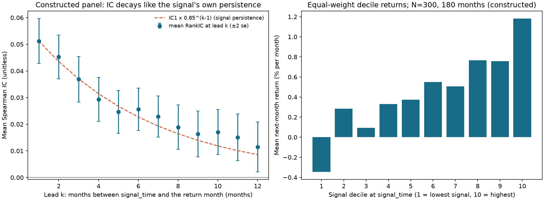
Figure 23-1: IC decay and decile returns in a constructed panel. The constructed panel has N=300 assets over 180 months. The signal is a heavy-tailed AR(1) process with autocorrelation 0.85. Next-period return is β⋅signal (β=0.004), plus a market component and heavy-tailed noise. The left plot shows average Rank IC by lead k (the single-period return in month k after the signal month-end), with error bars at ±2 standard errors; the orange dashed line starts at the first sample Rank IC and multiplies it by 0.85k−1. It borrows the Pearson-IC decay shape in the linear model of Section 6.7 as an order-of-magnitude reference, not an exact decay theorem for Rank IC in a heavy-tailed finite panel. The measured values are near this reference curve, slightly higher at long horizons but within the error bars. The right plot shows equal-weighted average monthly return by decile, which rises roughly monotonically from bucket 1 to bucket 10. Constructed data; mechanism demonstration.
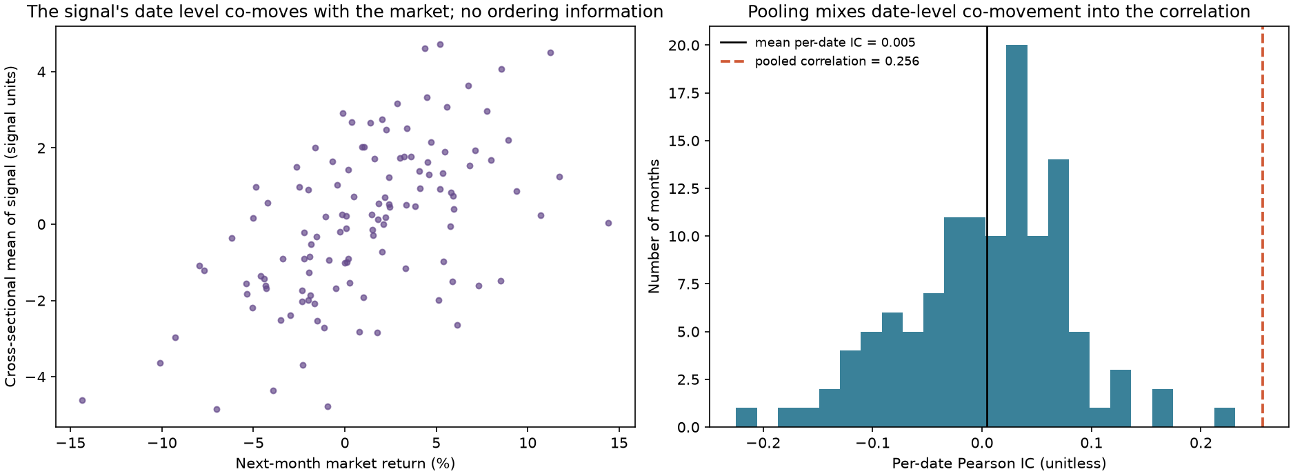
Figure 23-2: Pooled correlation and per-date IC. In this construction, the signal equals “within-date noise” plus a “date-level component.” The date-level component has a 0.5 correlation with next-month market returns; returns contain only the market component and noise unrelated to the signal. Each point in the left plot is a month, with next-month market return (%) on the horizontal axis and the cross-sectional mean signal for that month on the vertical axis; they move together. The right plot is a histogram of per-date IC over 120 months. The black line marks the mean, 0.005, and the orange dashed line marks pooled correlation, 0.256. The pooled correlation lies far outside the IC distribution because it measures date-level co-movement, not assets' ranking skill.
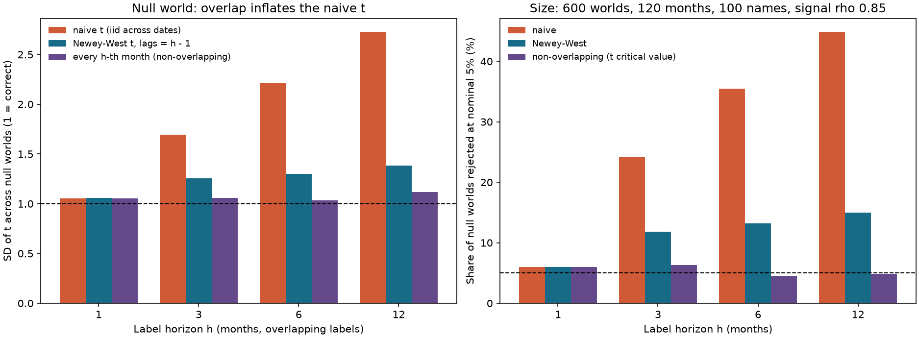
Figure 23-3: The size of three t statistics with overlapping labels. In a null world where returns and signals are independent, the construction has 120 months, 100 assets, signal autocorrelation 0.85, and 600 replications. The left plot shows the standard deviation of t statistics; the dashed line at 1 is a standard-normal/asymptotic reference. A finite-sample Student statistic need not have standard deviation exactly 1. The right plot shows the actual rejection rate for a nominal 5% test. The three bars represent the naive test (treating monthly IC as independent), Newey–West with lag h−1, and a sample that takes every hth month (nonoverlapping, using the t-distribution critical value). At h=12, the naive t statistic has standard deviation 2.7 and a 45% rejection rate. Newey–West reduces these to 1.38 and 15%, still above 5%. The nonoverlapping sample restores a rate near 5%, at the cost of using only T/h observations.
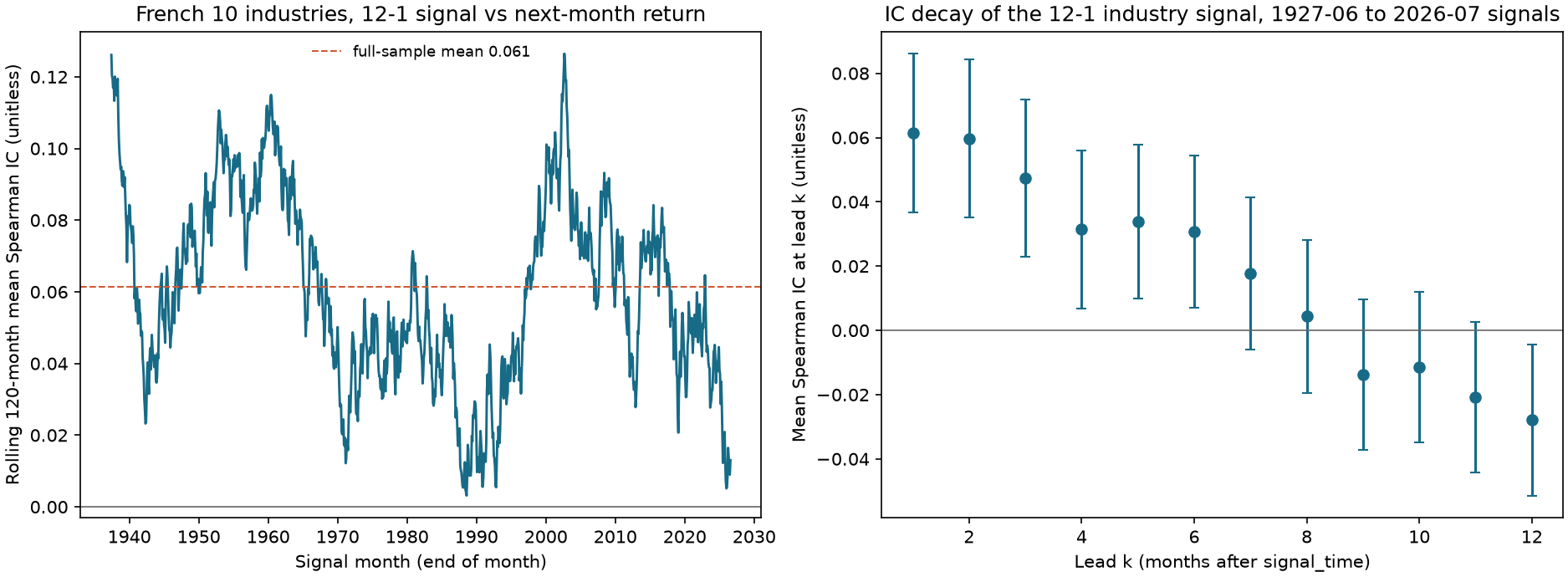
Figure 23-4: Rank IC and decay for a 12-1 signal on the 10 French industries. The left plot shows a rolling 120-month average Rank IC (horizontal axis: signal month-end); the orange line is the full-sample mean of 0.061. The right plot shows mean Rank IC at each lead, with error bars at ±2 Newey–West standard errors (lag 0). The rolling IC varies widely by period, from near zero to above 0.12. Average IC is positive for the first 6 months, turns negative starting in month 9, and reaches −0.028 (t=−2.37) at month 12. But that negative value should not be treated as a significant reversal when selecting among 12 leads: the two-sided Bonferroni threshold for M=12 is Φ−1(1−0.05/(2×12))≈2.865. The sample consists of 10 revised industry portfolios, not executable trades.
11. Historical market example
Data and definitions. Use the same frozen value-weighted monthly returns for the French 10 industry portfolios as in Chapter 22 (ZIP SHA-256 ebd937a4b995d821867aeb956a96f09a666386f38fa82516b7d1767ee4a49ae5; processed CSV SHA-256 3b097d810c295d64eedfa1ece7067ff2a0707f5ca90e33935df9949251f70950; 1,202 months from 1926-07 through 2026-08, in decimal simple returns per month; source and license are documented in Chapter 22 and data/manifests/french_industries_2026-10-05.json). Signal si,t: at month-end t, the compounded return over the prior 11 months from t−11 through t−1 (12-1, excluding the current month). Label: the simple return for the next month, t+1. The cross-section has N=10 industries; 1,190 months have both signal and label (1927-06 through 2026-07). This previews Chapter 25; here it demonstrates cross-sectional tools and is not a conclusion about momentum.
per-date Rank IC. Full-sample mean Rank IC is 0.0615 (standard deviation 0.425, hit rate 55.5%, t=4.99, Newey–West lag 0, T=1190). By subperiod: 1927-06 through 1963-12, 0.0868 (t=4.41, 439 months); 1964-01 through 1999-12, 0.0505 (t=2.45, 432 months); and 2000-01 through 2026-07, 0.0414 (t=1.70, 319 months). The last period is exactly the holdout evaluation from Chapter 22, with the same t=1.70. The standard deviation of monthly IC is large, 0.425, because each cross-section has only 10 assets. The approximate sampling standard error of monthly Rank IC is 1/9=0.33, so it is meaningful only after aggregating many months.
IC decay. Mean Rank IC for leads 1 through 12 is 0.0615, 0.0597, 0.0474, 0.0315, 0.0338, 0.0307, 0.0178, 0.0044, −0.0137, −0.0114, −0.0208, and −0.0279. The corresponding t statistics are 4.99, 4.84, 3.88, 2.56, 2.82, 2.59, 1.50, 0.37, −1.17, −0.98, −1.77, and −2.37. In this sample, mean IC is positive for the first six leads, while later point estimates are near zero or negative. These are sample associations in the same revised history, not a general “effective holding period.” Choosing among 12 leads is a multiple-comparison problem. The reported t statistics all use HAC lag 0, whose independent-date/calibration assumption still needs to be checked. Do not generalize the decay relationship from the stable AR linear model in Section 6.7 to real signals.
Quintile portfolios (two industries per bucket). Average next-month returns for buckets 1 through 5 are 0.759%, 0.890%, 0.981%, 1.101%, and 1.278% per month, increasing monotonically. The mean long-short return (bucket 5 minus bucket 1, with two industries equally weighted in each leg) is 0.519% per month, with t=3.64 when months are treated as independent. Mean target-weight turnover is 0.904 (two assets per leg, gross exposure 2; on average, about 45% of gross exposure is replaced each month). The mean membership turnover of bucket 5 is 22.9%.
Fama–MacBeth. Standardize the signal within each date using the population-form standard deviation and fit yi,t=at+btzi,t+ei,t each month, regressing the label on the standardized signal with an intercept. The average slope is bˉ=0.1686% per month per one standard deviation of signal, with Newey–West (lag 0) t=3.35. The mean intercept is 1.00%, the industry's average monthly return. The identity b^t=ICtσy,t holds across all 1,190 months with maximum absolute error below 10−15. The two t statistics differ (4.99 for IC and 3.35 for FM) because FM gives more weight to months with higher σy,t.
What this example shows and does not show. It shows that one signal can be measured through per-date IC, quantile portfolios, and FM slopes, with all three giving a positive direction but different significance; that the IC series varies widely across periods; and that a decay curve describes lead associations in this sample but does not directly set a tradable horizon. It does not show that the finding is tradable: 10 industry portfolios are revised published returns, not execution prices, and Chapter 22 only used assumed costs for illustration. Nor does it show that inference is robust: the cross-section has only 10 assets, subperiod t statistics differ, and the summary over 12 leads involves multiple testing. The same data have been used repeatedly in Chapter 22, so do not treat this t statistic as independent evidence.
12. Common mistakes
Mistake 1: Treating a correlation pooled across dates as IC. In the two-date example in Section 8.4, per-date IC is +1 and −1 (mean 0), while pooled correlation is 0.891. In the 120-month constructed example in Figure 23-2, pooled correlation is 0.256 while mean per-date IC is 0.005.
import numpy as np
import pandas as pd
from quant_course.factor_research import ic_series, ic_summary
rng = np.random.default_rng(5)
months, names = 120, 200
level = rng.standard_normal(months) # date-level driver
signal = pd.DataFrame(rng.standard_normal((months, names)) + 2 * level[:, None],
index=pd.period_range("2010-01", periods=months, freq="M"))
label = pd.DataFrame(0.045 * level[:, None] + 0.08 * rng.standard_normal((months, names)), index=signal.index)
pooled = np.corrcoef(signal.to_numpy().ravel(), label.to_numpy().ravel())[0, 1]
per_date = ic_summary(ic_series(signal, label, method="pearson")["ic"])
assert pooled > 0.2andabs(per_date.mean) < 0.02andabs(per_date.t_naive) < 3# ordering has no informationprint(round(pooled, 3), round(per_date.mean, 4), round(per_date.t_naive, 2))
Mistake 2: Breaking ties by row order. If you use “ordinal ranking” (argsort), assigning four tied signals to buckets depends on column order. Reordering the same data changes the portfolio.
import numpy as np
from quant_course.factor_research import quantile_bucket
x = np.array([0.0, 0.0, 0.0, 0.0, 1.0, 2.0, 3.0, 4.0])
average = quantile_bucket(x, 4)
reordered = quantile_bucket(x[::-1], 4)[::-1]
np.testing.assert_array_equal(average, reordered) # average-rank rule: order-independent
ordinal = np.argsort(np.argsort(x, kind="stable"), kind="stable") # ordinal ranks 0..7 break ties by position
ordinal_rev = np.argsort(np.argsort(x[::-1], kind="stable"), kind="stable")[::-1]
bucket_ord = lambda ranks: (4 * (ranks + 0.5) // 8).astype(int) + 1assertnot np.array_equal(bucket_ord(ordinal), bucket_ord(ordinal_rev)) # ordinal rule: depends on column orderprint(average.tolist(), bucket_ord(ordinal).tolist(), bucket_ord(ordinal_rev).tolist())
Mistake 3: Ranking the full table before dropping NaN, or filling NaN with zero before ranking. In the first case, ranks include assets that were later dropped. In the second, missing assets are treated as if they had a zero signal. The library functions rank within the valid pairs.
Mistake 4: Shifting the label by one month (look-ahead). Using the same month's return as a prediction label (conceptually k=0, a parameter the current lead_return rejects) includes already realized information. The example deliberately pairs the signal directly with same-month returns to demonstrate the error. In the example below, the constructed same-month return is correlated 0.7 with the signal, while the next month is entirely unrelated.
import numpy as np
import pandas as pd
from quant_course.factor_research import ic_series, ic_summary, lead_return
rng = np.random.default_rng(9)
idx = pd.period_range("2010-01", periods=120, freq="M")
returns = pd.DataFrame(0.08 * rng.standard_normal((120, 100)), index=idx)
signal = returns.mul(0.7).add(0.08 * rng.standard_normal((120, 100)) * 0.714) # built FROM this month's return (a leak)
same_month = ic_summary(ic_series(signal, returns, method="pearson")["ic"])
next_month = ic_summary(ic_series(signal, lead_return(returns, 1), method="pearson")["ic"])
assert same_month.mean > 0.5andabs(next_month.t_naive) < 3print(round(same_month.mean, 3), round(next_month.mean, 4))
Mistake 5: Using a naive t statistic with overlapping labels. In a null world with signal autocorrelation 0.85 and T=120, the naive rejection rate is about 24% for h=3 and 45% for h=12 (Figure 23-3). Remedy: use a nonoverlapping sample or at least Newey–West, recognizing that it remains optimistic (rejection rate 12–15%).
Mistake 6: Bucketing on full-sample quantiles. If cut points use the full panel, an early date's bucket depends on future data. quantile_bucket calculates separately for each date. Applying pd.qcut to an entire long-form panel would make this mistake.
Mistake 7: Using market capitalization or a universe from a later date. The cap used for value weights and the stock universe must reflect versions known at signal_time. Using market capitalization or delisting status that became available after month-end is look-ahead. The time-field tables in Chapter 24 and Project 4 list each field's available_at.
Mistake 8: Reading “significant t” as “profitable return.” In the constructed panel, the decile long-short gross return is 1.525% per month with t=10.4, but monthly target-weight turnover is 1.43 at gross exposure 2. At 10 bp per unit, the proxy cost is about 14 bp per month, only a fraction of the gross return. In the historical industry example, a high-turnover variant would consume more than half its gross return (Chapter 22). The cost share depends on signal persistence and must be reported alongside gross return.
13. Applications in quantitative research
Research table for the signal layer. Project 4's (multifactor strategy) research interface can be represented as a long-form table with primary key (date, security_id): raw feature, within-date percentile, bucket, next-month return, h-month label, industry, and market capitalization. The current implementation uses date-by-asset panels and separate metadata; the teaching long-form example is not an existing export file. Input features, industry, and market capitalization need records showing availability and ingestion before the cutoff. Ex post labels mark the evaluation interval and need not be available on the signal date. All functions in this chapter use this table as their input/output model.
Complete chain on a constructed panel (chapter experiment). The panel has N=300, T=180, and an AR(1) signal with ρ=0.85 and true IC1≈0.050. Results: mean Pearson IC 0.0501 (t=12.1, hit rate 83.8%); Rank IC 0.0512 (t=12.1). The plotted Rank-IC decay is compared with the reference shape 0.85k−1. Section 6.7 gives a Pearson-IC law for its specified linear model, not an exact Rank-IC law for this heavy-tailed finite panel. Equal-weight decile long-short return is 1.525% per month (t=10.4); equal-weight quintile return is 0.999%; market-cap-weighted quintile return is 0.836% (t=4.90); and signal-proportional return at gross exposure 2 is 1.042% (t=12.2). For the same IC, gross returns differ by more than 20% and t statistics by a factor of 2.5 across the three weighting schemes. This is why a claim that a “factor works” cannot omit the weighting rule. The z/N portfolio's mean return is 0.401% per month, the same as the Fama–MacBeth mean slope of 0.4013% (identity in Section 6.4). After adding a pure-noise signal, its FM slope has t=−1.0 and the true-signal slope is unchanged.
Project 4 constraints. (1) Report per-date IC and Rank IC, IC decay, quantile monotonicity, and turnover for each factor. (2) For overlapping labels, use nonoverlapping observations or report Newey–West as well. (3) Put missing-value and tie rules in the configuration. (4) Put long-short weights, gross exposure, and the cost convention in the configuration. (5) Record every experiment in Chapter 22's ledger. The signal-layer work in this chapter does not establish a strategy's return after costs.
13.1 Project 4 acceptance scope and tradable subspace
Layer
Current acceptance entrypoint and scope
Use in this chapter
A5 signal preparation
qa/a5/codex_followup_fixes/acceptance.md: constructed PIT, same-date processing, signal contract; missing real EV-bridge fields must not default to zero
Reads the feature and date contract; does not accept a complete strategy
A6 ledger interface
qa/a6/codex_resume/acceptance.md: constructed prices, listing filters, delisting, and ledger integration
Reads execution constraints; filtering after full-universe neutralization still leaves residual exposure
Cost sensitivity is a constructed experiment, not real alpha or capacity
A four-asset counterexample shows why filtering is not re-optimization. Industry 1 has weights (0.3,−0.3) on A and B; industry 2 has weights (0.2,−0.2) on C and D. Before filtering, each industry's weights sum to zero, total net exposure is 0, and gross exposure is 1. If B is untradable and set to zero, the resulting weights are (0.3,0,0.2,−0.2). Industry 1 exposure is 0.3, net exposure is 0.3, and gross exposure is 0.7. Even if scaled by 1/0.7 to restore gross exposure to 1, industry 1 and net exposure remain 3/7, not zero.
A complete Project 4 run must reconstruct or project weights over the assets tradable at that time, then check final nonzero weights for industry exposure, net exposure, gross exposure, single-asset caps, budget/cash, and all other prespecified constraints. If the feasible set is empty, define a fallback; do not claim that filtering preserves neutrality. A6 has already recorded this open interface. This chapter example gives readers a counterexample and checks; it did not change the shared optimizer or run new empirical work. Complete P4 methods, implementation, real data, and trading validation remain in the later project queue.
14. Chapter summary
Cross-sectional research turns “many assets on the same date” into testable quantities: rank within each date (ranks, percentiles, quantile buckets), measure prediction within each date (IC and Rank IC), and then treat dates as the observations for aggregation. Pooled correlation mixes in co-movement in date-level averages. In the specified constructed model, overlapping labels and persistent signals make the IC series autocorrelated; the long-run effective sample size is T/VIF. Other data-generating processes need separate checks. We connect prediction to holding with weights: a signal-proportional portfolio earns IC×σy, while quantile portfolios depend on bucket and weighting rules. In the specified model, signal persistence relates to IC decay; actual turnover also depends on weights and the universe. Fama–MacBeth expresses average return per unit of signal with a standard error, but its weighting differs from IC. In the historical French industry data, the same signal has a consistent direction across per-date IC, quantile portfolios, and FM, while significance varies by measure and period. Scope limits: the constructed panel demonstrates a mechanism; a 10-industry cross-section is small; French data are revised history; and this chapter measures costs only through turnover, so it does not draw strategy conclusions.
15. Exercises
23-E01 (conceptual) Why is the signal time month-end and why does the label begin in the following month? List the five time fields that a monthly research table must identify, and state which two require a strict ordering.
23-E02 (by hand) For the date-level cross-section x=(4,2,2,NaN,9,7,2,5,7), calculate average ranks, percentiles, and bucket numbers for q=3.
23-E03 (by hand) Five assets have signal s=(1,2,3,4,12) and next-period return y=(0.03,0.01,0.05,0.04,−0.06). Calculate Pearson IC and Rank IC, and explain the difference.
23-E04 (derivation) Prove that without ties, ∑(ri−rˉ)2=n(n2−1)/12, and use it to derive Spearman's formula 1−6∑d2/(n(n2−1)).
23-E05 (by hand) Two dates with three assets each. A: s=(1,2,3), y=(0.01,0.02,0.03). B: s=(5,6,7), y=(0.07,0.06,0.05). Calculate per-date IC, its mean, and the pooled correlation; use the law of total covariance to explain which term accounts for the difference.
23-E06 (by hand) Four assets have s=(1,3,5,7) and y=(0.02,0.01,0.05,0.04). Calculate z and verify that N1∑ziyi=IC×σy.
23-E07 (by hand) Two months, eight assets, and q=4. Month 1 signals: (3,1,8,5,6,2,7,4); month 2 signals: (3,2,8,1,6,5,7,4). Next-period returns for month 1: (0.03,0.00,0.06,0.02,0.04,0.01,0.05,0.02); for month 2: (0.02,−0.01,0.05,0.00,0.03,0.02,0.04,0.01). Calculate each month's long-short return, target-weight turnover, and the membership replacement rate in each of the two buckets. If the cost is 10 bp per unit of turnover, what is the net return in month 2?
23-E08 (calculation) Using the long-run approximation in Section 6.8, let signal autocorrelation be ρ=0.9, label horizon h=4, and T=240 months. Calculate VIF, neff, the adjusted value of a naive t=3.1, and the VIF and adjusted t recovered in population by Newey–West with h−1=3 lags.
23-E09 (interpretation) A signal has AR(1) coefficient 0.9. What is its half-life? If a signal's IC half-life is only one month, how would you choose a rebalancing frequency, and why?
23-R01 (pairs and dates; further practice) Redo Section 3.1: give Nsignal,t, npair,t, IC, and Tvalid for all three dates, and calculate the time-series standard error. Why can you not use ranks from the full signal set or fill February with zero? What does HAC lag 1 mean in the currently compressed series?
23-R03 (model conditions; further practice) Under the specified large-cross-section dependence model in Section 6.8, calculate finite-period VIF and equivalent date count for ρ=0.85 and −0.5 with T=120,h=3. Explain which conclusions do not generalize to arbitrary IC series.
23-R02 (portfolio and interface; further practice) For Section 7.1, report the raw and standardized FM slopes, the gross exposure of z/N, and the scaling to gross exposure 2. Then, for Section 13.1 after filtering out B, check industry, net, and gross exposure. Which of these steps can establish cost-adjusted alpha?
16. Programming exercises
23-P01 Write a function that takes a date-by-asset panel and returns the average next-month return for five buckets and the long-short return, using quantile_bucket and lead_return. Verify that the five buckets are monotonic and the long-short return is positive on constructed data. It must handle NaN and ties without error. Acceptance: one assertion for each of the three input types.
23-P02 On a constructed panel, calculate per-date Pearson IC and pooled correlation. Create a case where the signal's date-level component co-moves with the market, then verify that pooled correlation is much larger than mean per-date IC. Acceptance: pooled correlation >0.2 and absolute mean IC <0.02.
23-P03 Simulate a null world with an AR(1) signal (ρ=0.85) and independent returns, using h=3 overlapping labels. Compare rejection rates for naive t, Newey–West with lag 2, and a nonoverlapping sample. Acceptance: naive rejection rate is clearly above 5%, while the nonoverlapping rate is around 5%.
17. Challenge exercises
23-C01 (derivation) Under a bivariate normal assumption, derive the expected return of a q-quantile long-short portfolio, 2ICσyqφ(cq), and calculate qφ(cq) for q=3,5,10,20. Discuss the trade-off between long-short return and single-bucket sampling noise as buckets become narrower. Additional prerequisite: the conditional mean of a normal upper tail. Scoring: derivation 40 points, numerical values 30, trade-off discussion 30.
23-C02 (open-ended) Design the cross-sectional research table for the Value factor in Chapter 24. List each column name and source, the available_at rule, missing-value and tie rules, label interval, and industry and market-cap treatment. Give at least three tests that would make you conclude that a positive per-date IC is spurious. Scoring: time-field correctness 30 points, missing-value and tie rules 20, test design 30, treatment of overlapping labels and panel dependence 20.
18. Complete answers and reference implementations
23-E01 The chapter uses month-end signals based on information that was available and ingested before the cutoff, with actual execution after the signal. Five time objects: reporting period (period_end)/event time; publication and ingestion (available_at/ingested_at); signal_time (the current program uses the first instant of the next month as a strict cutoff); trade_time; and label start/end. Inputs must precede the signal cutoff, and signal_time < trade_time. Executable returns begin at the actual execution price. The current next-month month-end label is a research proxy under a hypothetical month-end execution assumption and includes a pre-execution return segment. A later calendar month alone does not establish correct execution timing.
23-E02 The valid values are (4,2,2,9,7,2,5,7), with n=8. Sorted values are 2,2,2,4,5,7,7,9: the three 2s occupy ranks 1, 2, and 3 and each receive average rank 2; 4 has rank 4; 5 has rank 5; the two 7s occupy ranks 6 and 7 and each receive 6.5; 9 has rank 8. The ranks, retaining NaN, are (4,2,2,NaN,8,6.5,2,5,6.5). Percentiles (r−1)/7 are (0.4286,0.1429,0.1429,NaN,1,0.7857,0.1429,0.5714,0.7857). For q=3, u~=(r−0.5)/8: rank 2 gives 0.1875, 4 gives 0.4375, 5 gives 0.5625, 6.5 gives 0.75, and 8 gives 0.9375. The values of 3u~ are 0.5625, 1.3125, 1.6875, 2.25, and 2.8125; bucket numbers are (2,1,1,NaN,3,3,1,2,3).
23-E03sˉ=4.4 and yˉ=0.014. Pearson IC is −0.865; the outlier signal of 12 corresponds to the lowest return, −0.06. Return ranks are (3,2,5,4,1) and signal ranks are (1,2,3,4,5). Thus d=(−2,0,−2,0,4), ∑d2=24, and ρS=1−6×24/(5×24)=1−1.2=−0.2. Pearson is sensitive to the outlier, which drives nearly all of the result; Rank IC considers only order, and −0.2 shows that the ordering relationship is also weak. If 12 is a real extreme signal, Pearson may capture it better; if it is a data error, Rank IC is more robust.
23-E04 Ranks are a permutation of 1,…,n, so rˉ=(n+1)/2 and ∑ri2=n(n+1)(2n+1)/6. Therefore, ∑(ri−rˉ)2=n(n+1)(2n+1)/6−n(n+1)2/4=n(n+1)[2(2n+1)−3(n+1)]/12=n(n+1)(n−1)/12=n(n2−1)/12. For the rest, see Section 6.2: define di=ri−qi, expand ∑di2, and use the equal sums of squares for the two permutations to obtain ∑(ri−rˉ)(qi−qˉ)=n(n2−1)/12−21∑di2. Dividing by n(n2−1)/12 gives the result.
23-E05 Date A has s and y moving together, so IC=+1. On B, s rises while y falls, so IC=−1. The mean is 0. In the pooled sample of six points, sˉ=4 and yˉ=0.04. For A, deviations are s−4=(−3,−2,−1) and y−0.04=(−0.03,−0.02,−0.01), with cross-product sum 0.09+0.04+0.01=0.14. For B, deviations are s−4=(1,2,3) and y−0.04=(0.03,0.02,0.01), with cross-product sum 0.03+0.04+0.03=0.10. Total cross-product is 0.24; divide by NT=6 for pooled covariance 0.04. The sums of squares are ∑(s−sˉ)2=28 and ∑(y−yˉ)2=0.0028. Pooled correlation is 0.24/28×0.0028=0.857. Decomposition: A's within-date covariance is ∑(s−2)(y−0.02)/3=0.02/3=0.00667, and B's is −0.00667, averaging to 0. Covariance between date means is 21[(2−4)(0.02−0.04)+(6−4)(0.06−0.04)]=21(0.04+0.04)=0.04. All pooled covariance comes from the second term: date B has higher signal and return levels.
23-E06sˉ=4, σs=(9+1+1+9)/4=5=2.236, and z=(−1.342,−0.447,0.447,1.342). Then 41∑ziyi=41(−0.02683−0.00447+0.02236+0.05367)=0.01118. Pearson IC is 0.7071. σy=41∑(y−0.03)2=(0.0001+0.0004+0.0004+0.0001)/4=0.015811, so IC×σy=0.011180. They match.
23-E07 Month 1 has q=4, n=8, and signals equal to ranks. Bucket assignment is ⌊4(2r−1)/16⌋+1: ranks 1 and 2 go to bucket 1; ranks 3 and 4 to bucket 2; ranks 5 and 6 to bucket 3; and ranks 7 and 8 to bucket 4. Bucket 4 in month 1 contains signals 7 and 8, assets 3 and 7, with returns 0.06 and 0.05 and mean 0.055. Bucket 1 contains signals 1 and 2, assets 2 and 6, with returns 0.00 and 0.01 and mean 0.005. Long-short return is 0.050. In month 2, bucket 4 has signals 7 and 8 (assets 3 and 7) with returns 0.05 and 0.04 and mean 0.045. Bucket 1 has signals 1 and 2 (assets 4 and 2) with returns 0.00 and −0.01 and mean −0.005. Long-short return is 0.050. Each leg uses weights ±0.5. Bucket 4 membership is unchanged; bucket 1 changes from assets 2 and 6 to assets 2 and 4. Target-weight turnover is 0.5+0.5=1.0; membership replacement is 0 for bucket 4 and 0.5 for bucket 1. Month 2 net return is 0.050−0.0010×1.0=0.049.
23-E08VIF=1+2[0.9×43+0.81×42+0.729×41]=1+2(0.675+0.405+0.18225)=3.5245; neff=240/3.5245=68.1; adjusted t=3.1/3.5245=1.65. The population Newey–West value is VIFNW=1+2[0.9×(43)2+0.81×(42)2+0.729×(41)2]=1+2(0.50625+0.2025+0.04556)=2.5086, giving t=3.1/2.5086=1.957. The naive t=3.1 looks highly significant; the adjusted value is about 1.65. Newey–West's 1.96 remains optimistic and sits near the 5% critical value.
23-E09 Under the stable linear construction in Section 6.7, half-life is ln0.5/ln0.9=6.58 months. If IC half-life is one month, forecast power halves within a month. Compare monthly rebalancing with shorter holding periods, while recognizing that turnover and fees may be higher. Decide using cost-adjusted returns under the frozen weighting rule, not IC alone. If half-life is longer (for example, 6.6 months), lower-frequency rebalancing is a candidate. Whether turnover falls and how much gross return is lost must be calculated under the specified weights, holding interval, rank changes, and costs; ρ alone does not guarantee it.
23-R01 Valid signal counts across the three dates are (4,4,4); paired counts are (3,4,4); IC values are (0.5,NaN,−1); and there are two valid dates. January must be re-ranked on A, C, and D, giving 0.5. Ranking all signals first and filtering later gives about 0.655. February's constant signal contains no ranking information, so correlation is undefined; filling it with zero changes the estimand. The mean is −0.25, sample standard deviation 1.06066, standard error 0.75, and naive t=−1/3. After compressing the array, lag 1 is one observation from January to March; it cannot be described as one month. Two dates do not support a statistical research conclusion.
23-R03 Finite-period VIF is 1+2∑j=12(1−j/120)ρj(1−j/3). For ρ=0.85, it is 2.59752778 and 120/VIF=46.1978. For ρ=−0.5, it is 0.50277778 and the equivalent date count is 238.6740. The earlier 2.615 and 45.9 are long-run approximations. With negative correlation, VIF is below 1, so do not state that “correlation” always means smaller standard errors or fewer effective dates. These results depend on the specified autocorrelation structure and do not solve the exact finite-cross-section problem with compounded labels and common shocks.
23-R02 Raw FM slopes are ±0.02; standardized slopes are ±0.02236; gross exposure of z/N is 0.89443. Multiplying by 5 gives gross exposure 2 and returns of ±0.05. Filtering out B gives industry sums (0.3,0), net exposure 0.3, and gross exposure 0.7. Scaling by 10/7 gives industry sums (3/7,0), net exposure 3/7, and gross exposure 1. Reconstruct the portfolio in the tradable universe and verify its final constraints. These are associations, gross returns, and constraint calculations; without actual costs and benchmark-risk attribution, none establishes cost-adjusted alpha.
23-P01 reference implementation
import numpy as np
import pandas as pd
from quant_course.factor_research import bucket_returns, lead_return
deffive_bucket_table(signal: pd.DataFrame, returns: pd.DataFrame) -> pd.Series:
table = bucket_returns(signal, lead_return(returns, 1), 5).dropna()
return table.mean()
rng = np.random.default_rng(11)
idx = pd.period_range("2010-01", periods=120, freq="M")
cols = [f"S{i:03d}"for i inrange(200)]
signal = pd.DataFrame(rng.standard_normal((120, 200)), index=idx, columns=cols)
returns = 0.004 * signal.shift(1) + pd.DataFrame(0.08 * rng.standard_normal((120, 200)), index=idx, columns=cols)
signal.iloc[5, :20] = np.nan # missing values
signal.iloc[7] = np.round(signal.iloc[7], 0) # many ties on one date
mean = five_bucket_table(signal, returns)
assert mean.loc[5] > mean.loc[1] and mean["LS"] > 0assert np.all(np.diff(mean.loc[[1, 2, 3, 4, 5]].to_numpy()) > -0.0015) # weakly increasing within noiseprint(mean.round(5).to_dict())
23-P02 reference implementation: See the code under Mistake 1 in Section 12, which reports pooled correlation alongside per-date IC. Set the coefficient on 2 * level to 0 and verify that both values are close to zero.
23-P03 reference implementation
import numpy as np
from scipy import stats
rng = np.random.default_rng(13)
months, names, h, rho, worlds = 120, 100, 3, 0.85, 400
naive, nw, non = [], [], []
for _ inrange(worlds):
total = months + h
z = np.empty((total, names)); z[0] = rng.standard_normal(names)
for t inrange(1, total):
z[t] = rho * z[t - 1] + np.sqrt(1 - rho**2) * rng.standard_normal(names)
r = 0.08 * rng.standard_normal((total, names))
label = sum(r[k:k + months] for k inrange(1, h + 1))
zs = z[:months] - z[:months].mean(axis=1, keepdims=True); ls = label - label.mean(axis=1, keepdims=True)
ic = (zs * ls).sum(axis=1) / np.sqrt((zs**2).sum(axis=1) * (ls**2).sum(axis=1))
naive.append(ic.mean() / (ic.std(ddof=1) / np.sqrt(months)))
d = ic - ic.mean(); lrv = d @ d / months + 2 * sum((1 - j / h) * (d[j:] @ d[:-j]) / months for j inrange(1, h))
nw.append(ic.mean() / np.sqrt(lrv / months))
sub = ic[::h]; non.append(sub.mean() / (sub.std(ddof=1) / np.sqrt(len(sub))))
reject = lambda a, c=1.96: float((np.abs(a) > c).mean())
assert reject(naive) > 0.15and reject(nw) > reject(non) and reject(non, stats.t.ppf(0.975, 39)) < 0.09print(reject(naive), reject(nw), reject(non, stats.t.ppf(0.975, 39)))
23-C01 From Section 4, E[y∣z]=μy+ICσyz. The upper-tail bucket is z>cq, with probability 1/q. Then E[z∣z>cq]=∫cq∞zφ(z)dz/(1/q)=qφ(cq), since ∫c∞zφ(z)dz=φ(c). The lower-tail mean is E[z∣z<−cq]=−qφ(cq). Therefore, long-short return is 2ICσyqφ(cq). Values of qφ(cq): for q=3, c=0.4307, φ=0.3636, giving 1.091; for q=5, c=0.8416, φ=0.2800, giving 1.400; for q=10, c=1.2816, φ=0.1755, giving 1.755; for q=20, c=1.6449, φ=0.1031, giving 2.063. Expected long-short return rises with q, but each bucket has fewer assets, N/q. The sampling standard error of a bucket mean is approximately σy/N/q (conditional variance approximately σy2(1−IC2)). With N=300,q=20, each bucket has 15 assets and its mean standard error is about 0.08/15=2.1%, far above the signal's expected contribution. Finer buckets raise expected long-short return, but also increase single-bucket noise and concentrate holdings in fewer assets. Compare the mean with its standard error to assess the long-short signal-to-noise ratio; noise alone does not determine the direction. The static normal formula contains no signal-transition process, so it cannot show that turnover must rise. Calculate actual turnover from dynamic ranks and weights. Fix q in the research plan. Score using the original three criteria.
23-C02 (scoring guide and reference). Suggested columns: date (month-end signal_time), security_id (permanent identifier), book_equity, and market_cap (latest version of each with available_at ≤ signal_time, using Chapter 13's select_pit_vintage); b_m (book equity/market cap; set to NaN and record reason when equity ≤0); industry (classification known at signal_time); rank_pct (within-date percentile, with a separate column for the within-industry version); bucket; label_1m; and label_3m (with intervals documented). Missing values: retain nonpositive equity and missing market cap as NaN; do not fill with zero. Ties: use average ranks. Three tests for a spurious positive IC: (1) delay available_at by one month and see whether IC disappears (timing test); (2) rank within industry and see whether IC remains positive (industry-effect test); (3) remove the largest 5% of assets by market cap and see whether IC remains positive (size-concentration test). A permutation test is another option. Score using the original four criteria.
19. Further reading
Must know: Petersen (2005 NBER working paper), abstract and introduction, then the section containing equations (8) and (9), to understand the assumptions behind Fama–MacBeth standard errors; useful for recognizing when FM t statistics are too large.
Should know: Jegadeesh and Titman (1993), Section I, on overlapping holding-period portfolios and turnover; read in depth in Chapter 25.
Should know: Chapter 22, Section 6, on multiple testing, and Chapter 15 on HAC.
Advanced: Original papers by Fama and MacBeth (1973), Newey and West (1987), and the chapters on IC and the Fundamental Law in Grinold and Kahn. These works have not been read for this chapter; obtain their texts before checking notation and conclusions.
Optional: Any publicly available factor research report; practice identifying when each column in its “research table” becomes available.
20. References
Citation keys and reading scope are listed in source_notes.md.
CH23_PETERSEN2005: Petersen, M. A. (2005/2006). “Estimating Standard Errors in Finance Panel Data Sets: Comparing Approaches.” NBER Working Paper 11280. Supports the discussion of Fama–MacBeth estimation and standard errors in Sections 5 and 6.6; the 2009 RFS final version has not been read.
CH23_JT1993: Jegadeesh, N., and Titman, S. (1993). “Returns to Buying Winners and Selling Losers.” Journal of Finance 48(1). Supports the discussion of overlapping holding periods.
CH23_SCIPY_RANKDATA: SciPy 1.18.1 documentation for scipy.stats.rankdata, supporting the average-rank definition.
FRENCH: Kenneth R. French Data Library, 10 Industry Portfolios (frozen snapshot).