CAPM and Asset Pricing

The argument begins with future payoffs discounted to today's prices using risk-adjusted weights. Under restrictive mean–variance equilibrium assumptions, CAPM reduces this risk adjustment to covariance exposure to the market portfolio. It provides a testable expected-return relation, rather than a prediction of next period's return or a trading instruction. Prerequisites: Chapter 5 on covariance and linear algebra, Chapter 8 on regression and robust inference, Chapter 10 on market contracts, and Chapter 11 on returns and compounding. You will distinguish no-arbitrage from equilibrium, derive CAPM by perturbing an efficient market portfolio, calculate beta and residuals by hand, reuse monthly regression code, and judge what an empirical deviation can establish.

1. Learning Objectives

Write a one-period stochastic discount factor pricing equation from future payoffs and explain how risk premiums affect prices. Distinguish no-arbitrage restrictions from equilibrium models. Calculate beta as covariance divided by market variance, and derive the Capital Asset Pricing Model (CAPM) from a local perturbation of a mean–variance efficient market portfolio. Distinguish the Capital Market Line (CML) from the Security Market Line (SML), and explain why zero beta does not mean zero total risk.

In practice, independently check the mean vector, covariance matrix, betas, and regression residuals of an explicitly constructed four-row example. The thin script corresponding to src/quant_course/asset_pricing.py reproduces a French monthly CAPM regression with fixed sources, SHA-256 hashes, frequency, and sample window. Its sample intercept is not tradable alpha. Successful work has consistent dimensions, hand-checkable examples, agreement between charts and script outputs, and an explicit account of what the case did not test.

2. Why Quants Need This

Before asking whether a signal predicts returns or makes money, quantitative research needs a relation between current prices and future payoffs. Ignoring state-dependent discounting treats assets with equal cash amounts in different states as equally valuable. Looking only at total volatility can mistake diversifiable variation for risk that the market must compensate. Asset pricing connects prices, exposures, and required expected returns, providing a clear null hypothesis for benchmarks, risk adjustment, and abnormal-return tests.

No-arbitrage excludes feasible free lunches without uniquely specifying every risk premium. CAPM adds investor choice, common expectations, risk-free borrowing and lending, and market clearing to obtain a particular market-beta relation. A good regression fit does not establish those assumptions. A nonzero historical intercept does not establish a financeable, executable strategy that remains profitable after costs.

Two constructed assets run through the chapter: their four-row mean total returns are equal, but their market betas are 0.5 and 1.5. Beta measures the direction and scale of market comovement; it does not rename a realized average as an expectation. Chapter 15 develops multiple factors. The historical case here is a single-factor market regression.

3. Intuition: In Which State Does the Asset Pay?

Consider a security paying EUR100 next period. Paying when incomes are ample and the marginal value of consumption is low can command a different current price from paying when incomes are strained and cash is most valuable. A state-independent average discount loses this distinction. A payoff received in a state with higher marginal value deserves more weight in its current price.

CAPM makes a strong simplification. In its one-period mean–variance world, investors adjust risk using the market portfolio and a risk-free asset. An asset that also falls when the market fares badly carries exposure that diversification cannot easily remove; equilibrium requires higher expected excess return. Beta summarizes that comovement. It does not measure every bad-state risk or guarantee that higher beta means a larger gain next period.

Asset A and Asset B both have a four-row mean total return of 7%, with excess-return betas of 0.5 and 1.5. If those rows were the complete probability distribution, they would not both satisfy the CAPM expected returns of 5% and 11% implied by a 2% risk-free rate and 8% expected market return. Here the rows are equally weighted teaching records, without a claim about long-run state probabilities. Sample means and model expectations are different objects; prediction and pricing require assumptions and evidence.

4. Mathematical Foundations: Units of Payoffs, Returns, and Risk

On a one-period timeline, today is $t$ and the next date is $t+1$. The terminal payoff $X_{t+1}$ and current price $P_t$ both have currency units. The simple total return $R_{t+1}=(X_{t+1}-P_t)/P_t=X_{t+1}/P_t-1$ is dimensionless; its gross return factor is $G_{t+1}=X_{t+1}/P_t=1+R_{t+1}$. Before displaying a percentage, check that an internal decimal such as 0.02 already means 2%; do not divide it by 100 again.

CAPM here relates expected simple returns over the same holding period, in the same currency and return convention. $R_f$ is the risk-free simple return and $\mathbb E[R_m]$ the expected market simple total return, rather than gross return factors. Monthly returns require monthly $R_f$ and a monthly market premium. Although dimensionless, monthly beta depends on frequency and the market proxy. An expectation under a model or population state distribution cannot be replaced by next period's realization.

For equally weighted observations $x_1,\ldots,x_n$, the sample mean is $\bar{x}=n^{-1}\sum_j x_j$ and sample variance is $s_x^2=(n-1)^{-1}\sum_j(x_j-\bar{x})^2$, with sample covariance defined similarly. Return variances and covariances have units of squared per-period return proportions. Their ratio gives dimensionless beta. For a return vector $R$ with $k$ entries, the mean vector $\mu$ has dimension $k$, and the $k\times k$ covariance matrix $\Sigma$ describes every pairwise comovement.

5. Formal Definitions: From General Pricing to Market Beta

A one-period stochastic discount factor (SDF), $m_{t+1}$, is a random, state-dependent weight converting terminal payoffs into current values. Under no-arbitrage and the required state-space conditions, write

The units of $m$ are current currency per unit of terminal currency; $mX$ has the same units as $P$. It maps a future payoff $X$ to a current price. States with high $m$ have higher marginal value: greater payoffs there command higher prices. This representation is more general than CAPM and does not by itself determine the market risk premium.

No-arbitrage excludes a feasible portfolio with nonpositive initial cost, nonnegative future payoff in every positive-probability state, and either strictly negative initial cost or strictly positive payoff in at least one state. We use a frictionless finite-state setting allowing cash borrowing and lending and linear combinations of trades. State probabilities are positive; prices define a consistent linear functional on attainable payoffs. In this setting, no-arbitrage is equivalent to strictly positive state prices and hence a strictly positive SDF, without requiring market completeness. Several positive SDFs may support the same traded prices, so no-arbitrage alone does not imply CAPM. Equilibrium also requires investors to optimize subject to budgets and preferences and markets to clear. CAPM is a model with explicit equilibrium assumptions.

Separate probabilities from pricing weights. In finite states $s=1,\ldots,S$, $p_s>0$ is the probability and $m_s$ the SDF in that state. The state price $q_s=p_sm_s$ is today's price of one terminal currency unit paid only in state s. When that state security cannot be traded separately, $q_s$ is an implicit weight supporting traded-asset prices. Thus

$p_s$ is dimensionless and sums to 1. Both $m_s$ and $q_s$ have units of current currency per terminal currency; $q_s$ need not sum to 1. A complete market has traded payoffs spanning the entire state-payoff space, yielding unique no-arbitrage state prices. In an incomplete market, several positive weight vectors can price all traded payoffs identically while valuing unspanned payoffs differently. A positive SDF establishes existence, without uniquely determining every expected risk premium.

The remaining chapter uses simple returns $R$, denoted $R_{t+1}$ in Section 4. To show the SDF identity, use gross return factors $G=1+R$, the risk-free simple return $r_f$ (that is, $R_f$), and its gross factor $G_f=1+r_f$. Normalize an asset's price to 1 to obtain $1=\mathbb E[mG]$. A risk-free terminal payment of 1 costs $\mathbb E[m]$, so $G_f=1/\mathbb E[m]$. Using $\mathbb E[mG]=\mathbb E[m]\mathbb E[G]+\operatorname{Cov}(m,G)$ gives

Because $G=1+R$, gross factors and simple returns differ only by 1: $\operatorname{Cov}(m,G)=\operatorname{Cov}(m,R)$ and $\mathbb E[G]-G_f=\mathbb E[R]-r_f$. Equivalently, $\mathbb E[R]-r_f=-\operatorname{Cov}(m,R)/\mathbb E[m]$. An asset paying less in high-SDF, high-marginal-value states requires greater expected return. The covariance uses the same one-period probability distribution. This general SDF interpretation precedes the additional restrictions on $m$ and the market portfolio that lead to a single CAPM beta.

Systematic risk is common risk that diversification alone cannot remove. Idiosyncratic risk is variation left over relative to the market or a specified factor model. A single-factor regression is

Beta is linear exposure of one-period asset excess returns to market excess returns. It depends on the sample, frequency, proxy, and estimator, rather than being an intrinsic asset constant. A fitted linear projection has in-sample residuals orthogonal to market excess returns, yet those residuals can have substantial variance. Zero beta means zero linear covariance, rather than zero total risk.

CAPM requires the following expected-return relation for any asset $i$:

Both sides are expected simple excess returns over the same interval, measured as returns per period; beta is dimensionless. For the market portfolio with $\beta_i=1$, the equation recovers its own risk premium. A zero-beta asset has zero CAPM expected excess return, while the market premium may remain nonzero and the asset may retain idiosyncratic risk. This is an equilibrium cross-sectional expectation restriction, rather than an identity for next period's realized returns.

The CML describes the expected return of efficient mixtures of the risk-free asset and market portfolio in mean–standard-deviation space:

Its slope is the market Sharpe ratio, the expected premium per unit of volatility. CML applies to efficient combinations of the risk-free asset and tangency market portfolio. SML relates expected return to beta for assets or portfolios under CAPM equilibrium. Their horizontal axes differ: total standard deviation for CML, market beta for SML. The two lines cannot be interchanged.

Equality of total- and excess-return covariances above concerns a conditional one-period distribution with $R_f$ known initially. RF can vary across historical months, so $\operatorname{Cov}(R_i-R_f,R_m-R_f)$ and $\operatorname{Cov}(R_i,R_m)$ need not coincide. Empirical interfaces therefore subtract each month's RF and define beta using excess returns. The fact that subtracting a constant leaves covariance unchanged does not justify dropping a time-varying RF column.

Distinguish the CAPM alpha target from its estimate. Theoretical expected alpha can be defined as $\alpha_i^{\ast}=\mathbb E[R_i-R_f]-\beta_i\mathbb E[R_m-R_f]$, which CAPM restricts to zero. The time-series intercept $\hat\alpha$ is estimated for a particular sample, market proxy, and model. Statistical rejection of zero neither realizes a future return nor establishes an executable strategy after financing and trading costs.

6. Derivation: Perturbing an Efficient Portfolio

Assume a one-period mean–variance setting: risky assets are tradable and divisible; the initially known risk-free return is constant across states; wealth weights satisfy $\sum_j w_j=1$. Investors borrow and lend at the same known $R_f$, share expected-return vectors and covariance matrices, and care only about mean and variance (or have jointly normal returns making this reduction appropriate). Market clearing aggregates their risky holdings into the market portfolio. Its variance and expected premium are positive. Locally, each risky-asset weight can be increased or decreased. Without these conditions, this derivation does not guarantee the conclusion.

Common expectations give investors the same mean–variance opportunity set. With borrowing and lending at the same risk-free rate, all select the same tangency risky portfolio; risk aversion changes its allocation against the risk-free asset. Risky-market clearing identifies that portfolio with the aggregate market. This theoretical market holds all investable risky assets at market-value weights; an index or French market factor is a proxy. Scaling the tangency allocation using $R_f$ is equivalent to choosing the risky portfolio with the highest Sharpe ratio.

Write the market portfolio $M$ with expected total return $\mu_m$, standard deviation $\sigma_m>0$, and excess return $a=\mu_m-R_f>0$. Reallocate a small weight $\varepsilon$ from it to asset $i$, retaining total weight 1:

The coefficients sum to 1, preserving the budget. Define the portfolio Sharpe ratio as $S(\varepsilon)=[\mu_p(\varepsilon)-R_f]/\sigma_p(\varepsilon)$. As the tangency portfolio of the common opportunity set, $\varepsilon=0$ locally maximizes Sharpe among fully invested risky portfolios. Both positive and negative small reallocations are feasible, so the derivative is zero. The mean derivative is $\mu_i-\mu_m$; the variance derivative at zero is $2[\operatorname{Cov}(R_i,R_m)-\sigma_m^2]$, and the standard-deviation derivative divides it by $2\sigma_m$. Apply the quotient rule before jumping to beta:

Here $S'(0)$ measures the marginal Sharpe change from reallocating a small wealth share, and $\sigma_p'(0)$ the marginal standard-deviation change. Substitute the second expression into the first, set $S'(0)=0$, and multiply by the positive $\sigma_m$:

This covariance uses total returns. Subtracting the same constant one-period risk-free return leaves covariance unchanged. The coefficient $a/\sigma_m^2$ follows from tangency Sharpe optimality, rather than an arbitrarily chosen historical regression coefficient.

Substitute $a=\mu_m-R_f$ and rearrange:

The ratio is market beta. The first line links marginal expected return to marginal common risk at the tangency optimum. The second cancels the market's own component. The third rewrites total returns as excess returns, since constant $R_f$ does not change covariance. This derives CAPM from equilibrium and efficiency without proving that real markets meet its assumptions. Different borrowing and lending rates, short-sale constraints, heterogeneous expectations, preferences beyond mean–variance, or an incomplete opportunity set can invalidate the common tangency portfolio or local first-order conditions.

7. Financial Meaning: Compensation for Marginal Common Risk

Diversification reduces the parts of security returns that do not move together. With many low-correlation assets, individual positive and negative residuals can offset. Exposure that falls with the entire market does not disappear by adding similar securities. CAPM therefore ties expected premiums to beta rather than total standard deviation. This remains conditional: omitted systematic factors can make market beta an incomplete risk description.

A beta above 1 indicates a larger historical linear excess-return response than the market itself; a negative beta indicates opposite sample linear comovement. Neither guarantees a return direction in a given period. Leverage usually increases equity sensitivity to underlying asset changes and can introduce financing constraints and bankruptcy risk. Scaling beta does not guarantee higher realized or risk-adjusted returns.

A zero-beta asset can have high variance. CAPM gives it zero expected market excess return, hence a required return of RF. This does not set the market premium to zero or eliminate total risk, loss probabilities, or holding costs. CML uses total volatility; SML uses market covariance. They describe different risk concepts.

8. Numerical Example

8.1 A Two-State Stochastic Discount Factor

8.2 Calculating Beta and Residuals from Four Rows

9. Python Implementation

Default Entry Point for This Reader Edition

From the accepted I3 reader package root, establish the documented environment, then run:

.venv/bin/python run_notebook.py notebooks/ch14_asset_pricing.ipynb

The default run checks four constructed return rows, betas, and residuals, then draws new CML/SML and beta-scatter charts using RF=2% and expected market return 8%. Both new PNGs go to runs/ch14_asset_pricing_<uuid>/. With RUN_FRENCH=False, the historical French regression and residual-chart branches are disabled: the default neither reads nor downloads market snapshots. The NoDur figures and tables in Sections 10–11 remain historical reading material.

The runner separately records kernel execution in a unique runs/execution_* directory, distinct from the chapter UUID method directory printed by the Notebook. Constructed execution checks computational interfaces; it produces no market research result, PIT forecast, or strategy return after costs. Chapter 14's historical NoDur inference uses HAC5; Chapter 15 and Project 2 historical main tables use HAC6. Keep point estimates and inference settings identifiable rather than altering intervals for superficial agreement. This batch inspected actual source without executing these Notebooks or rerunning historical regressions.

English Markdown for the Chapter 14 Notebook belongs to BIL23; this batch does not modify it. The CLI and old production tests below refer to the course working root. Readers need not restore production tests absent from the package.

Historical Course Working Root and Original Implementation

Core calculations are in asset_pricing.py: beta_from_covariance divides covariance by variance; fit_capm_excess returns estimates, fitted values, residuals, and (R^2) using single-regressor OLS identities; capm_expected_return applies the expected-return relation. Heteroskedasticity and autocorrelation consistent (HAC) inference uses the shared monthly fit_monthly_factor_model rather than a second engine. Missing or nonfinite inputs raise explicit errors, without silently dropping rows.

The ch14_asset_pricing.py script is a thin loading, reporting, and plotting layer. From the course root:

.venv/bin/python code/ch14_asset_pricing.py

For historical data, the manifest first verifies processed-file SHA-256 hashes; NoDur, Mkt-RF, and RF must then have consecutive PeriodIndex('M') months. Mkt-RF already subtracts RF, so the target subtracts it only once via NoDur - RF. Month labels do not establish information-availability, signal, or trade timestamps: this is not a backtest. HAC maxlags=5 means five adjacent monthly observation rows. Month ends separated by 28, 30, or 31 days are not converted to artificial equal-second timestamps. Inference depends on time-series approximations and bandwidth choices; significance alone does not establish alpha.

The CLI above belongs to historical course production, rather than the accepted I3 reader default. Programs 14-P01–P03 can be pasted independently at the working root after installing the course as documented. The local .venv/bin/python already imports quant_course directly, so no additional path bootstrap was added.

10. Visualization

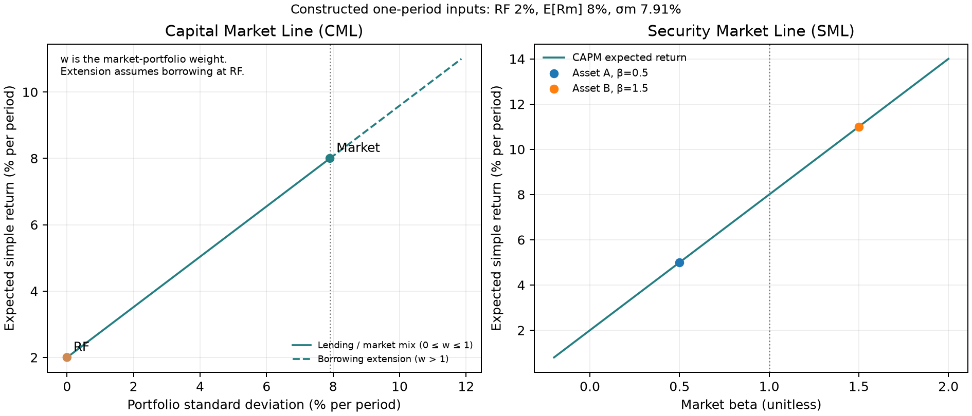
Left: horizontal axis is portfolio standard deviation (% per period), vertical axis expected simple return (% per period). Market weights from 0 to 1 combine the risk-free asset and market; the dashed extension assumes borrowing at RF for weights above 1. RF=2%, expected market return=8%, and market volatility about 7.91% are constructed inputs. The 7.91% uses ddof=0 on the four rows as an assumed model risk parameter, rather than Section 8's ddof=1 sample covariance risk estimate. It does not turn those rows into a true population state distribution. Right: horizontal axis is dimensionless beta, vertical axis model expected return, with endpoints calculated under the same assumptions. These are conditional model relations, rather than market observations.

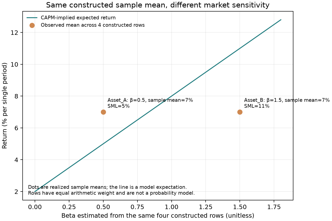
The horizontal axis shows beta estimated from the four constructed rows; the vertical axis shows their equally weighted mean total return. Orange points A and B both lie at 7%, while SML gives 5% and 11% at betas 0.5 and 1.5. The points are realized sample means and the line a constructed expectation model. Their gaps do not establish tradable alpha.

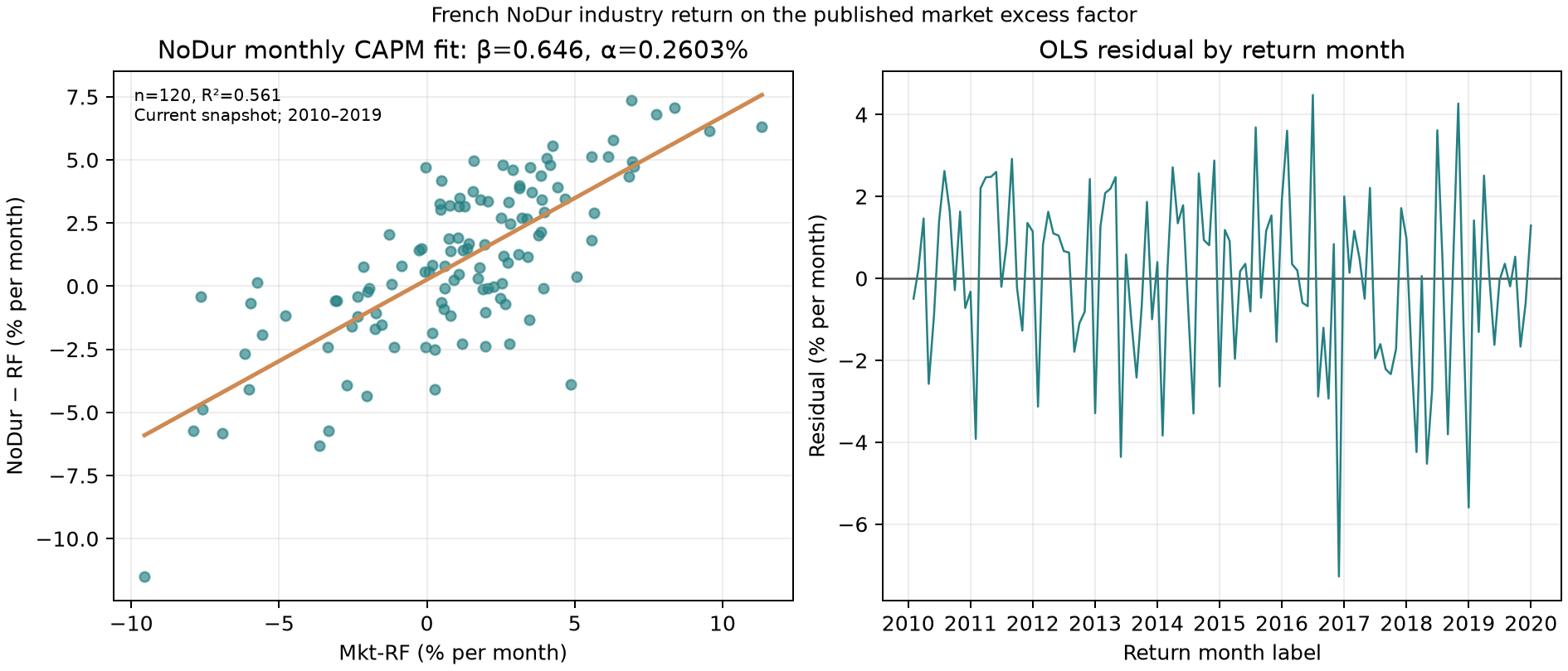
Left: Mkt-RF (% per month) horizontally and NoDur−RF (% per month) vertically; points are 120 published monthly rows from 2010–2019, with an OLS line fitted in that window. Right: return month horizontally and regression residual (% per month) vertically. These charts reveal linear association and residual time structure; one residual chart cannot establish model validity.

11. Real Market Example

The historical case estimates only a single market factor. NoDur is the value-weighted nondurables industry total return from French's monthly ten-industry portfolios; Mkt-RF is published market excess return; RF is the same-frequency one-month Treasury-bill proxy. The fixed window has 120 consecutive months, 2010-01 through 2019-12, with decimal processed-file hashes checked before calculation. See french_industries_2026-10-05.json and french_factors_2026-10-05.json: industry SHA-256 3b097d810c295d64eedfa1ece7067ff2a0707f5ca90e33935df9949251f70950; factor SHA-256 c19770a19a0ac47ad1c29074f57234570aeaa9725212cb4fa8146a2846c52814. The FF source declares CRSP database vintage month 202608. Both are current published snapshots from 2026, rather than point-in-time (PIT) data available in each historical month.

The equation is $NoDur_t-RF_t=\alpha+\beta(Mkt-RF)_t+\varepsilon_t$, using monthly decimal simple returns and dimensionless beta. Estimated monthly beta is 0.6456, with sample $R^2=0.5608$. Monthly intercept is 0.2603%, Bartlett HAC standard error 0.1926%, reference 95% interval [−0.1210%, 0.6417%], and reference two-sided $p=0.179$. HAC maxlags=5 counts consecutive monthly rows. Intervals and p-values are approximate under this estimation setup, rather than definitive judgments of beta or alpha.

Results are recorded in ch14_french_capm_2010_2019.json. This in-sample regression describes NoDur–market excess-return comovement. It does not test the complete aggregate-wealth market or include risk-free financing, costs, impact, capacity, or execution times. An intercept interval containing zero does not prove CAPM; an interval excluding zero would not alone establish a trading opportunity. Mean monthly NoDur total return is 1.0099%, RF 0.0427%, and excess return 0.9673%. These describe the fixed sample rather than next month's expectation.

12. Common Mistakes

One error subtracts RF from Mkt-RF again, producing $R_m-2R_f$ rather than standard market excess exposure. Another regresses raw asset total returns and labels its intercept CAPM alpha; RF changes the intercept and potentially the slope. The following historical frozen-data script checks hashes and compares correct and incorrect monthly betas and intercepts:

from pathlib import Path
import json
import sys
import statsmodels.api as sm

ROOT = Path.cwd()
sys.path.insert(0, str(ROOT / "src"))
from quant_course.factor_models import fit_monthly_factor_model
from quant_course.market_data import load_monthly_snapshot

industry_manifest = json.loads(
    (ROOT / "data/manifests/french_industries_2026-10-05.json").read_text()
)
factor_manifest = json.loads(
    (ROOT / "data/manifests/french_factors_2026-10-05.json").read_text()
)["datasets"]["ff3"]
industry = load_monthly_snapshot(
    ROOT / industry_manifest["processed_path"],
    industry_manifest["processed_sha256"], ["NoDur"]
)
factors = load_monthly_snapshot(
    ROOT / factor_manifest["processed_path"],
    factor_manifest["processed_sha256"], ["Mkt-RF", "RF"]
)
sample = industry.join(factors).loc["2010-01":"2019-12"]
correct = fit_monthly_factor_model(
    sample["NoDur"], sample[["Mkt-RF", "RF"]],
    factor_columns=("Mkt-RF",), hac_maxlags=5
)
wrong_factors = sample[["Mkt-RF", "RF"]].copy()
wrong_factors["Mkt-RF"] -= wrong_factors["RF"]
double_subtracted = fit_monthly_factor_model(
    sample["NoDur"], wrong_factors,
    factor_columns=("Mkt-RF",), hac_maxlags=5
)
raw_return_fit = sm.OLS(
    sample["NoDur"], sm.add_constant(sample["Mkt-RF"])
).fit()
print("correct beta:", correct.coefficient_table.loc["Mkt-RF", "estimate"])
print("beta after subtracting RF twice:", double_subtracted.coefficient_table.loc["Mkt-RF", "estimate"])
print("correct excess-return intercept:", correct.coefficient_table.loc["const", "estimate"])
print("raw-return intercept (not CAPM alpha):", raw_return_fit.params["const"])
assert round(correct.coefficient_table.loc["Mkt-RF", "estimate"], 6) == 0.645630
assert round(double_subtracted.coefficient_table.loc["Mkt-RF", "estimate"], 6) == 0.646460

In the frozen sample, correct beta is 0.645630, versus 0.646460 after subtracting RF twice. The correct monthly excess-return intercept is 0.2603%, versus 0.3036% for raw total returns. The latter is not the CAPM excess-return intercept. Use same-month NoDur - RF as the target and already-adjusted Mkt-RF directly as the regressor.

A third error substitutes $\hat\alpha$ or mean sample excess return for $\mathbb E[R_i]-R_f$. An estimated intercept and a realized path average can both reflect finite samples, revised data, proxy choice, structural changes, and residuals. Expectations concern a target population or equilibrium, without promising next period's realization.

A fourth error treats beta as all risk. A zero-beta asset can retain large residual variance; examine covariance, beta, total variance, and residuals together. A fifth announces a strategy from a significant intercept. Estimation does not automatically address selection, multiple testing, financing, taxes, impact, trading constraints, or when a signal became available.

Do not interpret a correlation regression as causal, or claim that ten industries or a common market proxy unambiguously test the complete market portfolio. Proxy coverage and mean–variance efficiency form a joint question, central to Roll's testability critique. This does not mean every CAPM test is invalid.

13. Quant Research Application

Define the research target first. Asking whether market beta explains cross-sectional mean returns is a pricing test; whether past beta predicts next month's return is a prediction test; whether a strategy earns investable net returns is a portfolio and execution test. Their dependent variables, estimation windows, information timing, and falsification conditions differ.

Preregister theoretical restrictions, proxy, frequency, sample window, and missing-data rules. Estimate beta only from returns available before the estimation date. Prediction tests need rolling or expanding windows, with estimates and signals available before trades. Strategy tests additionally define rebalancing, execution prices, borrowing and lending, costs, impact, short availability, and capacity. Use holdouts or rolling out-of-sample evaluation, report every tried model and asset, and retain insignificant results.

A falsifiable CAPM claim is that, for a specified tradable universe and preselected proxy, the cross-sectional mean excess-return slope on beta agrees with the market premium and intercept deviations fall within sampling uncertainty. Disagreement can reflect inapplicable assumptions, an inefficient proxy, noisy expected-return estimates, selection, or omitted risk. It does not automatically identify the cause. Conclusions must match the research estimand.

14. Chapter Summary

A one-period price is the expectation of future payoff weighted by an SDF. No-arbitrage permits a broader representation than CAPM. With mean–variance investors, common expectations and risk-free financing, market efficiency, and clearing, CAPM reduces compensation to market covariance beta. Local perturbation derivatives explain its origin; the assumptions show why it is not a law of nature.

Beta measures systematic linear comovement, rather than total risk or guaranteed future return. SML plots expected return against beta; CML plots efficient-portfolio expected return against standard deviation. Four rows suffice to hand-check the constructed means, betas, and residuals. The French case illustrates monthly regression and reference HAC inference, while one proxy, historical window, and intercept cannot alone confirm a theory or trading opportunity.

15. Exercises

Full answers appear in Section 18. Variables are same-interval simple returns, in decimals unless otherwise stated.

14-E01 | Pricing and prediction. In one sentence, distinguish one-period SDF pricing from the CAPM expected-return relation. What can neither guarantee alone?

14-E02 | Hand calculation of an SDF. Two equally likely states have discount factors 1.1 and 0.9. A security pays 0 and 2 respectively. Find its price, risk-free gross factor and simple return, and its own expected gross factor and simple return. Explain the premium's sign.

14-E03 | Risk and beta. Asset–market excess-return covariance is zero and market variance positive, while asset excess-return variance is 0.04. What CAPM expected excess return follows? Is total risk zero?

14-E04 | SML and CML. With $R_f=2\%$, $\mathbb E[R_m]=8\%$, and $\sigma_m=10\%$ ($\sigma_m$ is independently given here, rather than estimated from Section 8.2), find CAPM expected return for beta=1.5 and expected return for an efficient market/RF combination with 5% standard deviation. Identify each line.

14-E05 | Probabilities and state prices. Using Section 8.1, give both state prices and explain why probabilities alone do not price X. If only Y is traded, paying EUR100 in both states at a price of EUR100, are both state prices uniquely identified? Give two strictly positive weight vectors.

14-E06 | Two branches with equal volatility. Keep Section 5's RF=2%, expected market return 8%, and volatility 10%; set market weight to −0.5. Find expected portfolio return, standard deviation, and beta. Why does the positive-slope CML not give 5%?

16. Programming Exercises

14-P01 | Reproduce the constructed example. Call the core constructor and calculate sample means and covariance in order market, A excess, B excess. Obtain both betas as covariance ratios and fit both residuals. Check means 6%, 5%, 5%; betas 0.5 and 1.5; and residuals 1%, −2%, 2%, −1%.

14-P02 | Missing values. Replace a P01 observation with NaN and call fit_capm_excess. Test explicit rejection of nonfinite values, without silently dropping rows. Restore the data and confirm unchanged results.

14-P03 | Shared monthly estimation. Construct $y_t=0.001+1.2x_t+e_t$ from 60 observations on a monthly PeriodIndex('M') and estimate one factor with fit_monthly_factor_model. RF must be zero and present in the factor table; use HAC maxlags=5. Assert 60 observations, beta near 1.2, and residual mean near zero; print that the lag unit is monthly rows.

14-P04 | Historical data audit. Run the chapter script and read ch14_french_capm_2010_2019.json. Automatically check endpoints, 120 rows, monthly frequency, both file hashes, and the single-factor CAPM label. Do not relabel alpha_monthly as net strategy return.

17. Challenge Problems

14-C01 | Local perturbation derivation. Derive CAPM from tangency Sharpe maximization and feasible local perturbations. State the budget constraint, mean and variance derivatives, how the risk-free asset supports a common tangency portfolio, and where clearing identifies the market portfolio.

14-C02 | Zero beta with positive risk. Construct returns uncorrelated with market excess returns but having strictly positive variance. Explain the CAPM expected excess-return condition, its SML meaning, and risk conclusions that do not follow.

14-C03 | Estimated alpha and trading. A monthly intercept is 0.3% with HAC standard error 0.1%, reference (t=3). Give at least four further checks needed to move from a large estimated intercept to an implementable net trading opportunity.

14-C04 | Limits of the Roll critique. Explain why testing a linear return–beta relation with a market proxy also tests that proxy's mean–variance efficiency. Identify an overstatement the critique does not support and one design improvement.

18. Solutions / Solution Hints

14-E01 Answer. SDF pricing weights state payoffs to obtain today's price. CAPM expresses expected asset excess return as market beta times the expected market premium under specific equilibrium assumptions. Neither alone predicts a future month's realized return or establishes strategy profitability after financing and trading costs.

14-E02 Answer. Equal probabilities give $\mathbb E[m]=0.5(1.1+0.9)=1$, hence risk-free gross factor $G_f=1/\mathbb E[m]=1$ and simple return $r_f=G_f-1=0$. The security costs $P=\mathbb E[mX]=0.5(1.1\cdot0+0.9\cdot2)=0.9$. Its gross factor is 0 or $2/0.9=2.2222$, averaging $1.1111$; simple returns are -100% or 122.22%, with expectation 11.11%. Relative to $r_f=0$, its expected simple premium is 11.11 percentage points. It pays only in the lower-discount-factor state and therefore covaries negatively with $m$. This two-state example introduces no CAPM market-state assumption.

14-E03 Answer. Beta is $0/\operatorname{Var}(R_m-R_f)=0$, giving zero CAPM expected excess return without setting the market premium to zero. Asset variance is 0.04, standard deviation $\sqrt{0.04}=0.2$ or 20% per period, so total risk is positive. CAPM interprets it as risk lacking linear comovement with this proxy.

14-E04 Answer. SML gives $2\%+1.5(8\%-2\%)=11\%$. The efficient combination has market weight $w=\sigma_p/\sigma_m=5\%/10\%=0.5$ and CML expected return $2\%+0.5(8\%-2\%)=5\%$. The former prices beta 1.5; the latter relates standard deviation to return only for that efficient combination.

14-E05 Answer. $q=(0.45,0.55)$ and $P_X=0.45\times110+0.55\times90=99$ euros. Probability weights alone give EUR100, an expected payoff rather than risk-adjusted price. With only Y traded, the restriction is $100(q_1+q_2)=100$. Both $(0.45,0.55)$ and $(0.5,0.5)$ are strictly positive and satisfy it, but price unspanned X at EUR99 and EUR100. Y's no-arbitrage price therefore does not uniquely identify state prices. The two valuations of an untraded X are not themselves executable arbitrage.

14-E06 Answer. $\mathbb E[R_p]=2\%-0.5\times6\%=-1\%$ and $\sigma_p=|-0.5|\times10\%=5\%$; with constant RF, $\beta_p=w=-0.5$. SML consistently gives $2\%-0.5\times6\%=-1\%$. Positive-slope CML selects $w\ge0$, whereas this portfolio lies on the lower branch. Total standard deviation alone loses exposure direction.

14-P01 Reference implementation.

import numpy as np
from quant_course.asset_pricing import (
    constructed_two_asset_sample,
    fit_capm_excess,
)

sample = constructed_two_asset_sample()
returns = np.column_stack([
    sample["Mkt-RF"],
    sample["Asset_A"] - sample["RF"],
    sample["Asset_B"] - sample["RF"],
])
mean_vector = returns.mean(axis=0)
covariance = np.cov(returns, rowvar=False, ddof=1)
fit_a = fit_capm_excess(returns[:, 1], returns[:, 0])
fit_b = fit_capm_excess(returns[:, 2], returns[:, 0])
assert np.allclose(mean_vector, [0.06, 0.05, 0.05])
assert np.allclose(covariance[1:, 0] / covariance[0, 0], [0.5, 1.5])
assert np.allclose(fit_a.residuals, [0.01, -0.02, 0.02, -0.01])
assert np.allclose(fit_b.residuals, fit_a.residuals)

In squared decimal-return units the sample covariance is $\begin{bmatrix}.008333&.004167&.012500\\.004167&.002417&.006583\\.012500&.006583&.019083\end{bmatrix}$. The code uses order [Mkt-RF, Asset_A_excess, Asset_B_excess]; covariance and variance both use ddof=1, and their ratio gives beta.

14-P02 Reference test.

import numpy as np
import pytest
from quant_course.asset_pricing import constructed_two_asset_sample, fit_capm_excess

sample = constructed_two_asset_sample()
market = sample["Mkt-RF"].to_numpy()
asset = (sample["Asset_A"] - sample["RF"]).to_numpy(copy=True)
asset[1] = np.nan
with pytest.raises(ValueError, match="must be finite"):
    fit_capm_excess(asset, market)
asset[1] = 0.005
restored = fit_capm_excess(asset, market)
assert np.isclose(restored.beta, 0.5)
assert np.allclose(restored.residuals, [0.01, -0.02, 0.02, -0.01])

The test confirms explicit failure on a bad observation. Restoring the second excess return to 0.005 gives beta 0.5 and residuals [.01, -.02, .02, -.01]. Missing data do not authorize shortening the sample.

14-P03 Reference implementation.

import numpy as np
import pandas as pd
from quant_course.factor_models import fit_monthly_factor_model

month = pd.period_range("2015-01", periods=60, freq="M", name="month")
x = pd.Series(np.linspace(-0.08, 0.08, 60), index=month, name="Mkt-RF")
e = pd.Series(0.002 * np.sin(np.arange(60)), index=month)
rf = pd.Series(0.0, index=month, name="RF")
y = pd.Series(0.001 + 1.2 * x.to_numpy() + e.to_numpy(), index=month, name="asset")
fit = fit_monthly_factor_model(
    y,
    pd.concat([x, rf], axis=1),
    factor_columns=("Mkt-RF",),
    hac_maxlags=5,
)
assert fit.nobs == 60
assert abs(fit.coefficient_table.loc["Mkt-RF", "estimate"] - 1.2) < 0.01
assert abs(float(fit.residuals.mean())) < 1e-12
assert fit.hac_maxlags == 5  # five adjacent monthly observation rows

The deterministic sine error is not perfectly orthogonal to $x$, so beta need only be close to 1.2. Adjacent labels are consecutive monthly Periods, without artificial equal-second timestamps. HAC lag=5 means monthly rows. The helper subtracts RF once from asset returns; Mkt-RF already represents excess return and is not adjusted again.

14-P04 Reference checks. Command .venv/bin/python code/ch14_asset_pricing.py verifies manifest hashes before writing two QA JSONs and three charts. The frozen French record identifies 2010-01, 2019-12, n_months=120, frequency=monthly, and the single Mkt-RF factor. Hashes must match Section 11; investigate changed snapshots or processed files rather than altering expected values to hide differences. JSON alpha is a time-series intercept, never net strategy return.

14-C01 Reference derivation. Weights $(1-\varepsilon,\varepsilon)$ sum to 1, preserving the budget when reallocating a small position from M to i. The market tangency Sharpe ratio is locally maximal along these weights. The mean derivative is $\mu_i-\mu_m$, variance derivative $2[\operatorname{Cov}(R_i,R_m)-\sigma_m^2]$, and standard-deviation derivative divides the latter by $2\sigma_m$. Differentiate $S(\varepsilon)=[\mu_p(\varepsilon)-R_f]/\sigma_p(\varepsilon)$ and set the result to zero to obtain $0=(\mu_i-\mu_m)-[(\mu_m-R_f)/\sigma_m^2][\operatorname{Cov}(R_i,R_m)-\sigma_m^2]$. Rearranging yields $\mu_i-R_f=[\operatorname{Cov}(R_i,R_m)/\sigma_m^2]\cdot(\mu_m-R_f)$; the covariance ratio defines beta. Weight sums preserve the budget; common mean–variance expectations and RF produce a common tangency portfolio; clearing identifies it as the market. Infeasible two-sided perturbations, incomplete asset coverage, or heterogeneous expectations prevent this argument from identifying the relation.

14-C02 Reference construction. In four equally likely states, take market excess returns $X=(-1\%,-1\%,1\%,1\%)$ and asset excess returns $Y=(1\%,-1\%,1\%,-1\%)$. Both means are zero; state products $(-0.0001,0.0001,0.0001,-0.0001)$ average to zero covariance. Asset variance is $0.0001$ and standard deviation 1%, strictly positive. Positive market variance gives beta $0/\operatorname{Var}(X)=0$. Under CAPM, expected excess return is zero and SML gives RF at beta=0, while the market premium may remain nonzero. Total asset volatility is still 1%. This example does not establish zero volatility, no downside tails, or guaranteed principal.

14-C03 Reference answer. Check at least: (1) units, time zones, frequency, RF alignment, and whether the market factor already subtracts RF; (2) proxy coverage, omitted common risks, and parameter instability; (3) sample selection, all tried assets/frequencies/windows, holdouts, and multiple testing; (4) HAC bandwidth, residual dependence, structural changes, and small-sample approximations; (5) signal availability and executable trades; (6) fees, spreads, impact, financing, borrowing, taxes, and capacity; (7) incremental risk-adjusted results against a simple investable benchmark. Even a stable expected alpha requires an executable portfolio and risk budget. $t=3$ is a reference regression statistic, rather than proof of free arbitrage.

14-C04 Reference answer. Roll's original critique notes that if the proxy used as the market is not mean–variance efficient, departures from a linear mean–beta relation can reflect either pricing failure or proxy inefficiency. The exact theoretical market is not fully observable, so empirical tests impose joint restrictions on a proxy. This does not imply that all CAPM tests are invalid or all proxy results uninformative. Define the investable universe and proxy coverage explicitly, test proxy efficiency alongside cross-sectional restrictions, and report sensitivity across prespecified plausible proxies rather than selecting the most favorable result.

19. Further Reading

• Must Know: Read the Sharpe (1964) passages on mean–variance preferences, risk-free borrowing/lending, common expectations, efficient portfolios, and the return–beta relation. Source notes delimit actual reading. They support the theory without proving its assumptions hold in data.
• Should Know: Princeton FIN501 one-period pricing slides 43–66 explain SDFs, state prices, no-arbitrage, and additional beta-pricing restrictions. MIT OCW 15.401 CAPM slides 3–10, 15–16, 18–27 review diversification, SML/CML, and empirical issues.
• Advanced: Roll (1977), original abstract and market-portfolio testability argument, explains the proxy joint-test limit. Read the original paper for the full argument rather than relying only on this chapter.
• Optional: Markowitz (1952) publication metadata establish the historical source of mean–variance theory; the preparation did not read its full text page by page. Fama and French (2004) official abstract introduces a later empirical review, without this chapter restating the full paper.

20. References

1. Sharpe, W. F. (1964). “Capital Asset Prices: A Theory of Market Equilibrium under Conditions of Risk.” The Journal of Finance, 19(3), 425–442. Original article and publication metadata. Supports mean–variance assumptions, efficient portfolios, and market risk; actual reading scope is in source_notes.md.
2. Markowitz, H. (1952). “Portfolio Selection.” The Journal of Finance, 7(1), 77–91. Wiley metadata and DOI. Metadata only were checked, without full page-by-page reading.
3. Princeton FIN501. Lecture 02: One-Period Asset Pricing, slides 43–66. Supports general pricing kernels and SDFs; all technical conditions of the fundamental theorem are not developed here.
4. Lo, A. W. MIT OCW 15.401. The CAPM and APT, specified slides. See source notes for reading and formula-adaptation scope.
5. Roll, R. (1977). “A Critique of the Asset Pricing Theory’s Tests Part I: On Past and Potential Testability of the Theory.” Journal of Financial Economics, 4(2), 129–176. DOI, UCLA scan. This chapter uses metadata and the first-page abstract to explain the proxy joint-test limit.
6. Fama, E. F., and K. R. French (2004). “The Capital Asset Pricing Model: Theory and Evidence.” Journal of Economic Perspectives, 18(3), 25–46. AEA official page and abstract. Metadata and abstract only were checked.
7. statsmodels official OLS and robust covariance results documentation. It supports software calls, without selecting this study's model, HAC bandwidth, or economic interpretation.
8. Kenneth R. French Data Library. 10 Industry Portfolios, Fama/French Factors. See Section 11, source notes, and manifests for snapshot scope. Official methods do not confer historical PIT eligibility.