: Tree-Based Models

Author: Yuxiao Ma. The existing A8-B constructed implementation has been accepted within a limited scope and is pending formal integration; this does not mean that real research is complete. Core idea: trees approximate nonlinearities and interactions with piecewise-constant predictions; random forests reduce variance by averaging; gradient boosting iteratively repairs residuals along the negative gradient. Their depth, leaf size, number of rounds, and learning rate must all be selected using date-based validation inside the training data. Feature importance is a bounded diagnostic; economic conclusions still depend on a portfolio compared with benchmarks under the same accounting and costs. Prerequisites: the Chapter 38 pipeline (date-based walk-forward validation, label-availability times, and in-training tuning) and Chapter 39 regularized linear models (bias–variance and benchmark comparison). After completing this chapter, you should be able to hand-calculate an optimal split and two rounds of boosting; derive the random-forest variance formula; explain why built-in early stopping in sklearn 1.9.1 HistGradientBoosting cannot be used directly for a panel; compare tree and linear models on predictive metrics and after-cost results within the Chapter 38 pipeline; compute date-wise permutation importance and explain its limits with correlated features.

1. Chapter Objectives

1. Write down the split objective for a regression tree, derive “split gain $=\frac{n_Ln_R}{n}(\bar y_L-\bar y_R)^2$,” and hand-calculate a split for eight stocks.
2. Explain how depth and leaf sample size (min_samples_leaf) constrain tree variance, and identify which splits are infeasible under a given constraint.
3. Derive the variance of an average of $B$ trees with pairwise correlation $\rho$, $\rho\sigma^2+\frac{1-\rho}{B}\sigma^2$, and explain why random forests sample features at random.
4. Derive why each round of gradient boosting fits residuals under squared loss and how the learning rate shrinks each step; hand-calculate two rounds of boosting; explain how the HistGradientBoosting leaf value $-G/(H+\lambda)$ relates to Ridge shrinkage in Chapter 39.
5. Select depth, leaf size, and number of rounds (early stopping) by date within the training data, and explain why sklearn's built-in random holdout for early stopping leaks information in panels.
6. Compute date-wise permutation importance, compare it with mean decrease in impurity (MDI), and explain how correlated features, the sample period, and multiple comparisons affect it; explain SHAP's additivity and limitations.
7. Compare out-of-sample and after-cost performance for zero prediction, the training mean, OLS, Ridge, a single tree, a random forest, and gradient boosting on an interaction panel and the Chapter 39 linear panel; use the Project 6 v2 protocol for ablation and stability reporting.

Completion criteria: You can independently complete Sections 15–17; code/ch40_tree_models.py reproduces the numbers in Sections 8–10.

2. Why Quant Needs Tree Models

Linear models assume that each feature has a fixed slope with respect to expected returns. Two common departures in cross-sectional research are effects that vary with another feature (interactions—for example, a price-volume signal that works only for illiquid stocks) and non-monotone effects (both tails are unusual, while the middle is ordinary). Linear models require the researcher to add interaction and piecewise terms by hand, and the number of candidate combinations grows quickly with the number of features.

Tree models automatically search for “which feature and threshold should split the sample.” Gu, Kelly, and Xiu (2020) report higher out-of-sample $R^2$ for random forests and gradient-boosted trees than for linear benchmarks on monthly U.S. individual-stock data (see Sections 11 and 20 for the specific figures and review status). The same study also illustrates the costs: trees have many hyperparameters, are sensitive to the sample period, and can change their feature-importance rankings across training windows. This chapter checks these costs within the Chapter 38 pipeline: depth and number of rounds are selected only on date-based validation windows inside the training data; importance is computed on in-training validation windows; and economic value is compared with zero prediction, the training mean, and linear models using the same accounting and costs.

3. Intuition

There are eight stocks. Feature $x$ is the cross-sectional rank of the past five-day return (1 = largest decline, 8 = largest gain), and label $y$ is next week's return (%). These are constructed teaching values:

A depth-1 tree (a stump) asks one question: “Is $x\le s$?” It then predicts one constant on each side. At $s=4$, the left-side mean is −1%, the right-side mean is 2%, and the overall mean is 0.5%. Without a split, the sum of squared errors is 22; after the split it is $2+2=4$, a reduction of 18. Section 8 calculates each threshold; $s=4$ gives the largest reduction.

The boundary of this example: it has one feature and no independent validation set from later dates. A tree can keep splitting until each leaf contains one stock, reducing training error to 0. That zero training error reveals the risk of overfitting, but these eight rows cannot prove that the next week must be worse; evaluation requires validation or test data from later dates. Depth and leaf-size constraints, random-forest averaging, and the learning rate and number of boosting rounds all address the problem of splitting too finely.

4. Mathematical Setup

Prerequisites: Chapter 8 least squares (the mean minimizes squared error), Chapter 9 gradient descent, Chapter 39 bias–variance decomposition and the Ridge shrinkage factor $n/(n+\alpha)$, and Chapter 38 date-grouped walk-forward validation with $\text{label\_available\_at}\le\text{fit\_time}$. The clock in this chapter follows Chapter 38: signal_time is the close of $D_k$, trade_time is the close of $D_{k+1}$, and label_end $=$ label_available_at $=D_{k+1+h}$, where $h=5$.

5. Formal Definitions

Regression tree (CART). Recursive axis-aligned splits partition feature space into disjoint rectangular regions $R_1,\dots,R_J$, with a constant prediction in each region:

At each split, choose feature $j$ and threshold $s$, dividing node $S$ into $S_L=\{i:x_{ij}\le s\}$ and $S_R=\{i:x_{ij}>s\}$. The default squared_error criterion in sklearn 1.9.1 DecisionTreeRegressor chooses $(j,s)$ to minimize $\mathrm{SSE}(S_L)+\mathrm{SSE}(S_R)$; the leaf value is the mean of $y$ in that leaf. The algorithm is greedy, one level at a time, and is not guaranteed to find a global optimum. Not every rectangular partition can be represented by a recursive tree of a given depth. Trees address the need for linear models to specify interactions and thresholds by hand; the inputs are features and labels, and the output is a piecewise-constant prediction.

Depth and leaf samples. max_depth limits the number of splits from root to leaf, allowing at most $2^d$ leaves. min_samples_leaf requires each leaf to contain at least the specified number of training rows; a split that violates this condition is infeasible. Both constraints limit model complexity and therefore variance. In a panel, a row is one stock on one day, and rows from the same day are highly correlated. “1,000 rows” is far from 1,000 independent observations (see the effective sample discussion in Chapter 37), so leaf sizes generally need to be much larger than in nonfinancial applications.

Bagging and random forests. Bagging draws $B$ bootstrap samples from the training set and grows one tree on each; predictions are averaged. At each split, a random forest considers only a random subset of max_features, reducing dependence across trees. In sklearn 1.9.1, RandomForestRegressor defaults to max_features=1.0 (no feature subsampling, equivalent to bagging); max_samples controls how many rows each tree draws.

Gradient boosting. Starting from a constant $F_0$, each round fits a shallow tree $h_m$ to the negative gradient of the loss with respect to the current predictions, then adds it with a learning rate:

This extends Chapter 9 gradient descent from parameter space to “prediction-function” space: a tree approximates the direction of each step. sklearn 1.9.1 HistGradientBoostingRegressor (HGB) first bins each feature into at most 255 bins using training data, then searches for splits using sums of gradients and second derivatives within bins.

Learning rate and early stopping. The learning rate $\nu$ shrinks each step. A smaller step generally requires more rounds, while fitting less noise in each round. The number of rounds $M$ is a hyperparameter: too few underfit; too many fit noise. Early stopping halts when validation error no longer decreases. Validation must be held out by date from within the training rows; this chapter selects $M$ by recording validation error round by round on the inner date-based walk-forward folds in Chapter 38.

Mean decrease in impurity (MDI). For each feature, sum the weighted SSE reductions from all splits that use the feature, then normalize. sklearn's documentation refers to this as “Gini importance” and warns that it is biased toward features with many possible split values. It is computed on training data.

Permutation importance. On a validation set that was not used for fitting, shuffle a feature's values and measure the increase in loss:

where $X^{(\pi_r,j)}$ denotes column $j$ permuted according to permutation $\pi_r$ on repetition $r$. For the panel in this book, permutation is performed within each signal_time (cross-sectionally), never across dates, so date-level market conditions are preserved; the decline in daily Spearman IC is also reported. Group permutation applies the same row permutation to all columns in a group, preserving their joint distribution.

SHAP (Shapley additive explanations). Given a prediction $f(x)$, distribute $f(x)-E f(X)$ across features using Shapley values from cooperative game theory:

where $v(S)$ is the expected prediction when only the values of features in $S$ are known. Two common definitions of $v$ are the interventional form $v(S)=E\,f(x_S,X_{\bar S})$ (the omitted features $X_{\bar S}$ are sampled from the background joint marginal distribution, independently of fixed $x_S$; this does not mean that omitted columns are sampled independently of one another) and the conditional form $v(S)=E[f(X)\mid X_S=x_S]$. The definitions give different answers when features are correlated. The book's environment does not have the shap package installed; Section 8 computes exact Shapley values by enumerating a small example.

Ablation. A pre-registered comparison run that removes a feature group or swaps out a component, using the same folds, portfolio construction, and costs, to answer: “How much does this component contribute to out-of-sample results?”

6. Derivations

6.1 Leaf Values and Split Gain

The leaf value is the mean. A constant leaf prediction $c$ minimizes $\sum_{i\in S}(y_i-c)^2$. Differentiating with respect to $c$ gives $-2\sum(y_i-c)=0\Rightarrow c=\bar y_S$. This uses squared loss; under absolute loss, the leaf value is the median.

Within-group and between-group decomposition. Split parent node $S$ into $S_L$ and $S_R$, and let $\bar y$ be the parent mean. Add and subtract each side's mean before expanding (the cross term vanishes because $\sum_{i\in S_L}(y_i-\bar y_L)=0$):

Simplifying the between-group term. Since $\bar y=(n_L\bar y_L+n_R\bar y_R)/n$, $\bar y_L-\bar y=\frac{n_R}{n}(\bar y_L-\bar y_R)$ and $\bar y_R-\bar y=-\frac{n_L}{n}(\bar y_L-\bar y_R)$. Substituting gives:

Two implications follow. First, gain grows with the squared difference between the two means, but split comparisons must also include the sample-balance factor $n_Ln_R/n$; comparing only the mean difference is insufficient. Second, $n_Ln_R/n$ is largest when the two sides have equal sample sizes and is about 1 when one side has only one row. Isolating one extreme stock can still yield substantial gain, which is what min_samples_leaf is meant to guard against. For the Section 3 example at $s=4$, $\frac{4\cdot4}{8}(-1-2)^2=18$.

Decision use. The formula shows what a tree looks at: the product of the squared difference in group mean returns and the sample-balance weight. It does not look at slope or rank correlation. A feature useful for ranking but with a small difference in group means may never be selected.

6.2 Averaging Reduces Variance: $\rho\sigma^2+\frac{1-\rho}{B}\sigma^2$

Fix a feature point $x$. Treat each tree prediction $T_b(x)$ as a random variable (randomness comes from bootstrap sampling and feature sampling at splits). Assume the trees are identically distributed, each with variance $\sigma^2$, and every pair has correlation $\rho\ge0$. Then

The first step expands the variance of the sum into $B$ variances and $B(B-1)$ covariances, each covariance equal to $\rho\sigma^2$. As $B\to\infty$, the second term vanishes and variance approaches $\rho\sigma^2$: averaging many trees removes only the part on which trees differ, not the part they share. Random feature sampling may lower $\rho$, but it may also change the bias and variance of an individual tree; compare overall error. A smaller max_features is not guaranteed to be better. The formula matches Equation (15.1) in the second edition of ESL (see Section 20 for review status).

Financial interpretation: every tree sees the same chance market episode within a training window, so averaging cannot remove it. A longer sample, coarser leaves, or validation on a different window is needed to expose that error.

6.3 Gradient Boosting Fits Residuals Round by Round under Squared Loss

Initialization. $F_0=\arg\min_c\sum_iL(y_i,c)=\bar y$ (the same derivation as in Section 6.1).

Negative gradient. For $L(y,F)=\tfrac12(y-F)^2$, $-\partial L/\partial F=y-F$. At round $m$, the pseudo-residual is $r_{im}=y_i-F_{m-1}(x_i)$.

Fit and update. Fit a shallow tree $h_m$ to $\{(x_i,r_{im})\}$; its leaf value is the mean residual within the leaf (equivalently, the least-squares solution under squared loss). Then update $F_m=F_{m-1}+\nu h_m$.

Learning-rate shrinkage. Suppose each round selects the same partition. Let the initial mean residual in leaf $R$ be $\bar r_R^{(0)}$. One round reduces every row's residual by $\nu\bar r_R^{(0)}$, so the leaf's mean residual becomes $(1-\nu)\bar r_R^{(0)}$; by induction, after $m$ rounds it is $(1-\nu)^m\bar r_R^{(0)}$. With $\nu=1$, the residual is removed in one step; with $\nu=0.1$, about $0.9^{10}\approx35\%$ remains after 10 rounds. This is a special case (the partition changes across rounds in real boosting). It illustrates that a small learning rate breaks one large correction into many small ones, each of which can be rejected by subsequent validation error. That is why “learning rate × number of rounds” must be tuned jointly.

HGB leaf value. sklearn 1.9.1 HGB computes a leaf value using the gradient sum $G=\sum g_i$ and Hessian sum $H=\sum h_i$ as $-G/(H+\lambda)$, then multiplies it by the learning rate (source: compute_node_value in splitting.pyx and shrinkage in grower.py; see D06 and Section 20). Under squared loss $L=\tfrac12(y-F)^2$, $g_i=F-y_i=-r_i$ and $h_i=1$:

l2_regularization $=\lambda$ multiplies the mean residual in the leaf by $n_R/(n_R+\lambda)$, which has the same form as the Ridge shrinkage factor $n/(n+\alpha)$ under orthogonal design in Chapter 39: smaller leaves are shrunk more.

6.4 Early Stopping Must Hold Out by Date

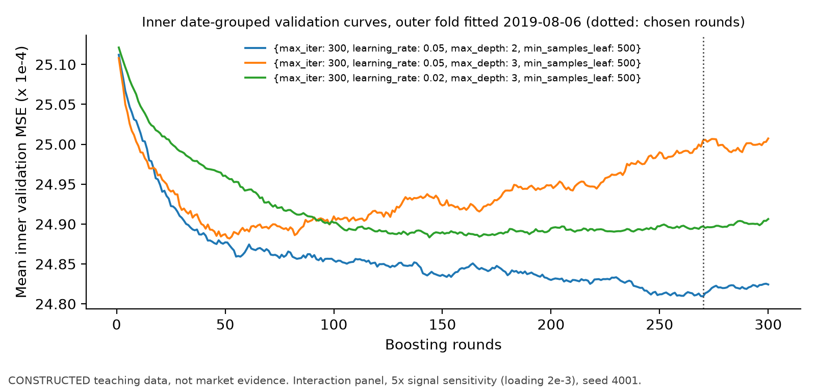
When the training set has more than 10,000 rows, HGB's early_stopping="auto" turns early stopping on and uses train_test_split (test_size=validation_fraction) to randomly sample 10% of training rows as a validation set (local source lines 533–581). This creates two problems in panels: other stocks from the same day remain in the training set, so validation rows share that day's market shock with training rows; and five-day label intervals overlap, with adjacent signal dates sharing four days of returns, so the validation labels have almost been “seen” on the training side. Random row holdout breaks the time-out-of-sample validation design and may understate error. In the constructed panel in Section 12.1, it indeed stops too late, but this is not a theorem that it always selects more rounds or always worsens test results. The correct approach is to disable built-in early stopping, treat the number of rounds as a hyperparameter, record validation MSE at every round (staged_predict) on the inner date-based walk-forward folds in Chapter 38, choose the minimum of the mean curve, and refit on all outer-training rows using that number of rounds. Evaluate the outer test window only once. Section 12.1 compares the numbers from random early stopping and date-based early stopping.

6.5 Permutation Importance with Correlated Features

Let $x_2=x_1$ (the columns are identical), and suppose the fitted model uses only $x_1$ (this is an assumption about the fitted model; when gains tie, feature search, random state, and implementation conventions can affect the result, so one cannot assume the first column is selected). Permuting $x_2$ alone leaves the prediction unchanged, so $I_2=0$; under the predictor, labels, and MSE specified in Section 8.4, permuting $x_1$ damages useful prediction, so $I_1>0$. Merely reading a column does not guarantee a loss increase on every validation set. The same information receives a high or low rank depending on which column the model happened to use. If a model uses the columns as substitutable predictive proxies (for example, in some forests), the unpermuted column may preserve information and dilute single-column importance. Reading both columns does not itself guarantee this. Joint permutation measures the loss change under the group perturbation. The sign and substitution behavior depend on the model, validation distribution, and loss. For example, take two rows with $x_1=x_2=(-1,1)$, $y=(0,0)$, and a fixed $f=x_1-x_2$. Baseline MSE is zero; swapping either column alone gives MSE 4, while swapping both together leaves MSE zero. This algebraic counterexample does not claim that a forest fitted to these data would learn that function.

The second issue is extrapolation. If $x_1$ and $x_2$ are highly, but not perfectly, correlated, permuting $x_1$ alone can create combinations that do not occur in reality (high $x_1$ with low $x_2$). The model's predictions on these points have no support in the training data, so the importance measures its behavior in unfamiliar regions. Strobl et al. (2008) proposed conditional importance to address this issue (see Section 20 for review status).

Third, importance depends on the sample period: the result belongs to the window and fold used to compute it. In this book, importance used for any selection is computed only on in-training validation windows; importance computed on an outer test window is a post hoc diagnostic and must not feed back into that window or any later model, parameter, or feature selection.

6.6 Shapley-Value Additivity and Limitations

Take $p=2$, an interventional definition, and a single background point $b$: $v(\varnothing)=f(b)$, $v(\{1\})=f(x_1,b_2)$, $v(\{2\})=f(b_1,x_2)$, and $v(\{1,2\})=f(x)$. Substituting into the definition gives:

Adding gives $\phi_1+\phi_2=v(\{1,2\})-v(\varnothing)=f(x)-f(b)$, the additivity property (local accuracy). Limitations: (1) SHAP explains the model, not the world. If the model uses only $x_1$, the interventional Shapley value for $x_2$ is 0 even if $x_2$ contains the same information in the data. (2) Interventional and conditional definitions allocate credit differently for correlated features; neither automatically equals “economic importance.” (3) Interaction credit is split according to a rule (see the $f=2x_1x_2$ example in Section 8.4); the split follows from the axioms, not from discovering a mechanism. (4) Like permutation importance, SHAP depends on the sample period and background distribution and can vary across folds. (5) It does not provide a causal explanation: a “large SHAP value” does not mean that changing the feature would change returns.

7. Financial Interpretation

What trees capture. A tree predicts different mean returns on either side of a split and is well suited to conditional effects: a signal may work only for a particular class of stocks. For example, in the interaction panel in Section 8, $q_1$ has a loading only when $q_2>0$. A linear model can learn only an average slope (about half the true conditional slope), while a tree can first split on $q_2$ and then on $q_1$. Whether such a structure exists or is stable in real markets requires empirical evidence; constructed data can demonstrate only the mechanism.

Effects of piecewise-constant predictions on portfolios. All stocks in a leaf receive the same prediction, creating many tied cross-sectional ranks. With shallow trees and large leaves, a dollar-neutral portfolio is effectively long and short across a few “buckets”; Spearman IC is less informative when there are many ties. Forests and boosting add many trees and reduce ties, but their predictions remain step functions.

Extrapolation. A feature value outside the training range falls into an outermost leaf, where the prediction remains constant; it does not extrapolate along a slope as a linear model would. In extreme markets, this can protect against amplified predictions while also hiding effects in a new region.

Turnover and costs. Tree predictions jump at thresholds: a small feature change across a split can move a prediction and portfolio weight by a full step. This can increase turnover; a small accuracy advantage may be erased by costs. Section 13 compares after-cost results using the same Chapter 29 accounting.

Implementability and timing. A strictly monotone transformation preserves training-point order and separable training partitions (ignoring floating-point effects, ties, and binning boundaries), but it does not guarantee identical predictions for new points after a nonlinear transformation. For training data $x=(0,2)$ and $y=(0,1)$, the original midpoint threshold is 1. On the nonnegative domain, the strictly increasing transform $g(x)=x^2$ changes the midpoint threshold to 2. At a new point $x=1.2$, the original tree predicts 1; after transformation, $1.44\le2$, so it predicts 0. A positive affine rescaling (for example, standardizing with a fixed training mean and positive standard deviation) preserves the corresponding midpoint. This does not mean that preprocessing can be done arbitrarily: winsorization by full-sample quantiles, bins fitted on the full sample, and HGB bins fitted on the full sample all let training data see the test-period distribution. Compute a cross-sectional rank only after the complete, contemporaneously available cross-section for that signal_time is ready; fit transformations and bins across time using training rows only.

8. Numerical Example

All numbers in this section are constructed for teaching. Sections 8.1–8.4 are hand calculations, checked against scikit-learn 1.9.1 by the hand-calculation portion of code/ch40_tree_models.py; Section 8.5 comes from the registered main simulations in the same script (seed and settings in its docstring and D08 of qa/a8/ch40_ch41_batch/DECISION_LOG.md). Section 8.6 is the D11 fivefold sensitivity added after seeing the main results, not a primary result specified in advance.

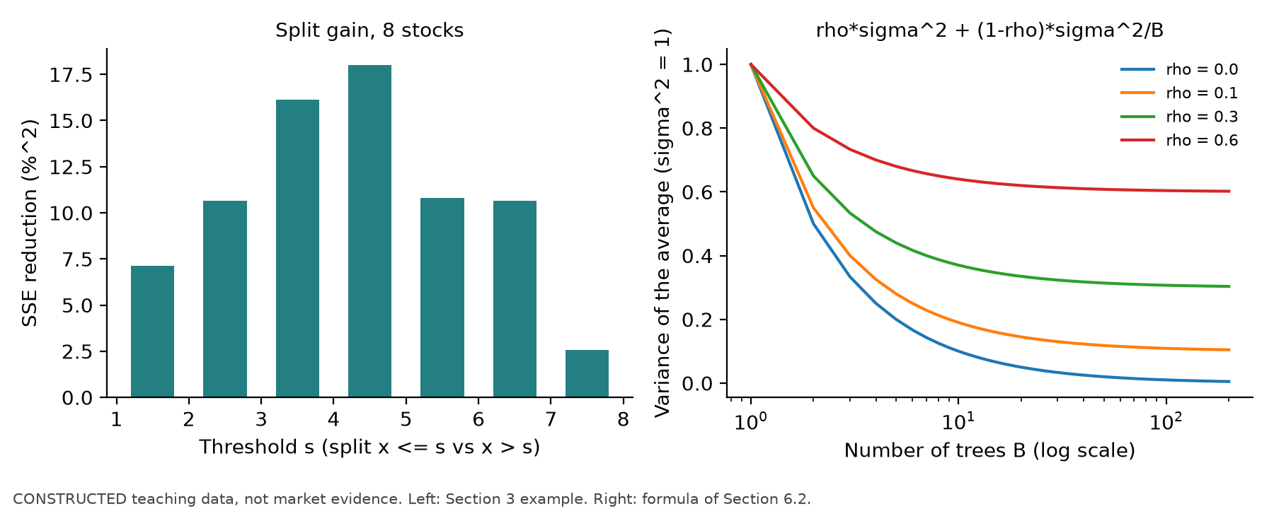
8.1 One Split: Calculate Each Threshold

Use the eight stocks from Section 3 (the unit of $y$ is %, the overall mean is 0.5, and $\mathrm{SSE}=22$):

The closed-form column uses $\frac{n_Ln_R}{n}(\bar y_L-\bar y_R)^2$. For example, at $s=1.5$, $\frac{7}{8}\times2.857^2=7.143$; at $s=4.5$, $\frac{16}{8}\times3^2=18$. The optimal threshold is 4.5 (sklearn places the threshold midway between adjacent values), with left-leaf value −1% and right-leaf value 2%. DecisionTreeRegressor(max_depth=1) returns the same threshold, 4.5, and leaf values $(-1,2)$. With min_samples_leaf=3, only $s\in\{3.5,4.5,5.5\}$ are feasible, and 4.5 remains optimal. If $y_8$ changes from 2 to 9, the optimal split becomes one that isolates stock 8; the leaf-size constraint then takes effect (see 40-E02 in Section 15).

8.2 Random-Forest Variance

Let $\sigma^2=1$ and $\rho=0.3$. For $B=1,10,100,\infty$, the variance of the average is $1,\ 0.37,\ 0.307,\ 0.3$. Increasing the forest from 10 to 100 trees reduces variance by only 0.063; the remaining 0.3 is determined by correlation. If random feature sampling lowers correlation to 0.1 at the cost of raising individual-tree variance to 1.2, then the limit as $B\to\infty$ is $0.1\times1.2=0.12$, much lower than 0.3. This arithmetic illustrates the random forest tradeoff: sacrifice individual-tree performance in exchange for lower correlation across trees.

8.3 Two Boosting Rounds with Learning Rate 0.5

Round 0: $F_0=\bar y=0.5$, residuals $r=(-2.5,-1.5,-1.5,-0.5,1.5,0.5,2.5,1.5)$, and training MSE $=22/8=2.75$.

Round 1: Find the best stump for the residuals. Because the residuals are $y$ minus a constant, the SSE reduction is the same as in Section 8.1; the optimal threshold remains 4.5. The mean residual is −1.5 in the left leaf and 1.5 in the right leaf. Thus $F_1=0.5+0.5\times(\mp1.5)$: predictions are −0.25 for the first four stocks and 1.25 for the last four. Training MSE is 1.0625.

Round 2: The new residuals are $(-1.75,-0.75,-0.75,0.25,0.75,-0.25,1.75,0.75)$. The optimal threshold is now 3.5: the left-leaf mean is $(-1.75-0.75-0.75)/3=-13/12$, and the right-leaf mean is $(0.25+0.75-0.25+1.75+0.75)/5=0.65$. Then $F_2=F_1+0.5\,h_2$: predictions for stocks 1–3 are $-0.25-13/24=-0.7917$, for stock 4 are $-0.25+0.325=0.075$, and for stocks 5–8 are 1.575. Training MSE is 0.5344.

The setup below produces exactly the same $F_2$ values on these eight points ($-0.791667,\dots,0.075,1.575,\dots$). Training MSE continues to fall in rounds 3 and 4, to 0.3205 and 0.2014. The number of rounds to keep must be decided by validation error outside the training window.

HistGradientBoostingRegressor(max_iter=2, learning_rate=0.5, max_leaf_nodes=2,
                              min_samples_leaf=1, early_stopping=False)

Leaf-value shrinkage. On the same data, with max_iter=1, learning_rate=1, max_depth=1, and l2_regularization=4, the residual sum in the left leaf is $-6$ for its four samples, giving a leaf value of $-6/(4+4)=-0.75$ and prediction $0.5-0.75=-0.25$; the right-leaf value is $+0.75$, giving prediction 1.25. sklearn returns $(-0.25,1.25)$. Without $\lambda$, the leaf values would be $\mp1.5$; $\lambda=4$ multiplies them by $4/8$.

8.4 Small Examples of Permutation Importance and Shapley Values

Twin features. There are four stocks on one day, with $x_1=(-1.5,-0.5,0.5,1.5)$, $x_2=x_1$, and $y=(-0.9,-0.4,0.2,1.1)$ (%). Suppose the fitted model uses only $x_1$: $f=0.6x_1$. The baseline MSE is 0.015. Use the fixed permutation “shift forward by two positions,” $\pi=(3,4,1,2)$:

• Permute $x_1$ only: predictions become $0.6\times(0.5,1.5,-1.5,-0.5)$, MSE is 1.575, and importance is 1.560.
• Permute $x_2$ only: predictions do not change, so importance is 0.
• Permute both columns together: importance is 1.560.

$x_2$ contains exactly the same information as $x_1$, yet its importance is 0. If the model happened to select $x_2$, the ranking would reverse.

Shapley values for an interaction. Let $f(x_1,x_2)=2x_1x_2$, $x=(1,1)$, and background point $b=(0,0)$. Then $v(\varnothing)=0$, $v(\{1\})=f(1,0)=0$, $v(\{2\})=0$, and $v(\{1,2\})=2$. Thus $\phi_1=\tfrac12\cdot0+\tfrac12\cdot2=1$, $\phi_2=1$, and their sum is $2=f(x)-f(b)$. The interaction contribution is split equally. For the twin-feature model $f=0.6x_1$ at $x=(1.5,1.5)$, $\phi=(0.9,0)$.

8.5 Run Results: Interaction and Linear Panels (Main Results)

Setup (registered before the run). There are 40 assets and 1,260 trading days. The conditional mean for the interaction panel is $0.0004\times g$, where $g=q_1\mathbf 1\{q_2>0\}+0.8(|q_3|-\sqrt{2/\pi})$. The linear panel reuses the Chapter 39 generator, with conditional mean $0.0004\times(q_1+0.5q_2+0.25q_3)$. Each panel has 20 pure-noise features plus rev_5, mom_60_5, and vol_20, for a total of 26 columns. The setup uses $h=5$, a one-day lag, an expanding outer window (at least 504 days of training, 63 test days per fold, 12 folds), and the last two 63-day validation windows for inner tuning; the grid matches Project 6 v2. Portfolios are dollar neutral, rebalance every five signal dates, and trade at the next close. Each row's $R^2_{\text{OS}}$ is relative to the training mean; IC is the mean daily Spearman IC over the test period.

Zero prediction and the training-mean portfolio are both flat. Every model has negative $R^2_{\text{OS}}$ relative to the training mean. In the interaction panel, all absolute IC Newey–West $t$-statistics are below 1.2; the largest in the linear panel is 1.35. The tree models did not find the interaction signal. Inner validation reflects this too: in 11 of 12 folds, gradient boosting selects only 1–14 rounds, and the single tree selects the shallowest depth, 2, in 8 folds. Signal scale matters: in the interaction panel, the standard deviation of $g$ is about 0.86, the daily standard deviation of the conditional mean is about $3.4\times10^{-4}$, and idiosyncratic volatility is 2% per day. If the signal is approximated as constant over five days and idiosyncratic shocks as independent, ignoring compounding and the heterogeneous-beta common term, the cumulative signal-to-idiosyncratic-noise variance ratio is approximately $5(3.4\times10^{-4}/0.02)^2=0.001445$, or 0.145% (on the order of 0.1%). This is a conditional scale calculation, not a measured five-day statistic from the panel. This run did not detect the interaction over 12 folds and roughly 750 test days. In the linear panel, the single tree's Sharpe of 0.59 comes from a few favorable splits in 12 folds; its IC is only 0.0057 and should not be treated as evidence.

8.6 Signal-Strength Sensitivity (Added Post Hoc, D11)

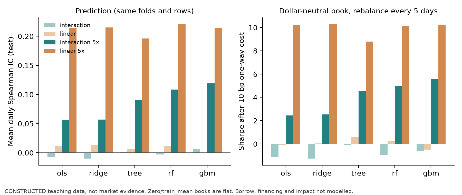
After viewing the main results, both panels' loadings were increased fivefold to 0.002 to show what trees can do when a signal is detectable; all other settings were unchanged. This was not a registered main result. Sharpes of 5–10 are far beyond any realistic strategy and indicate only an excessively strong constructed signal.

On the interaction panel, tree models achieve about twice the IC of linear models: linear models can use only the average slope on $q_1$ (theoretically half the conditional slope) and the linear parts of $q_2$ and $q_3$ (the linear projection of $|q_3|$ is 0); trees can first split on $q_2$, then on $q_1$, and split both tails of $q_3$. On the linear panel, Ridge, gradient boosting, and the forest are nearly identical, while the single tree is clearly worse: approximating a straight line with steps requires many splits, and the selected depth—usually 2–4 in 11 of the 12 folds—is not enough. On the interaction panel, inner validation selects 20–270 rounds for gradient boosting (mostly 39–112), far more than the 1–14 rounds in the main result. When a signal is present, validation error keeps declining and early stopping selects more rounds.

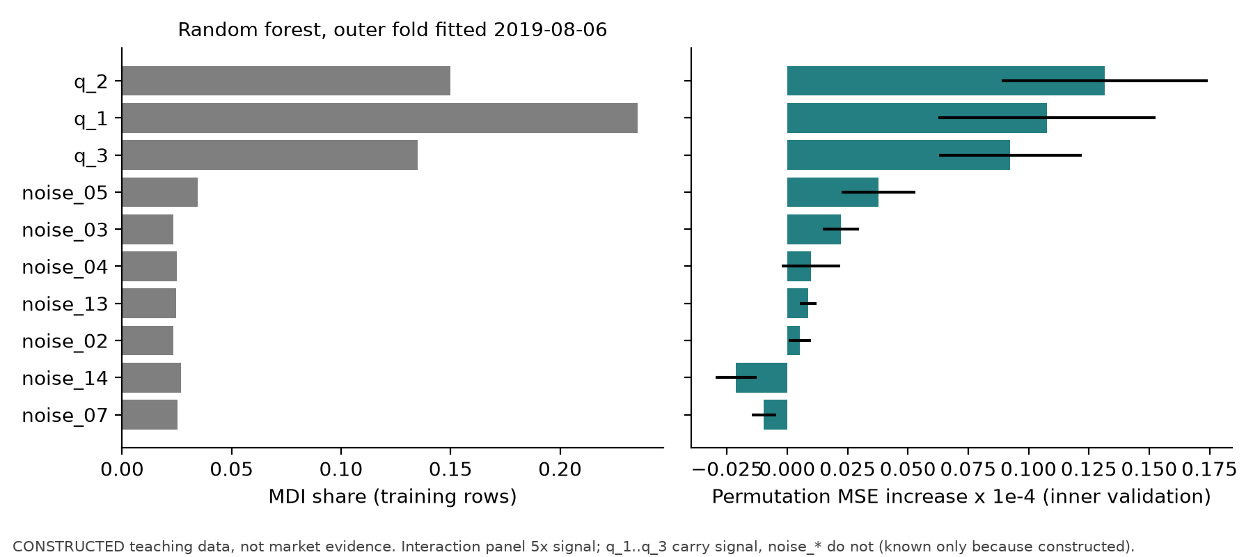
Importance. On the fivefold interaction panel, the random forest computes date-wise permutation importance on the last inner validation window of each fold (three repeats). Mean MSE increases for $q_1,q_2,q_3$ are $0.318,0.099,0.061\times10^{-4}$; across 12 folds, $q_1$ and $q_3$ enter the top 10 every time and $q_2$ does so in 11 folds. The pure-noise feature noise_05 also enters the top 10 in 7 folds, with a mean increase of $0.018\times10^{-4}$. The mean Spearman correlation between importance rankings in adjacent folds is 0.36 (range 0.05–0.64). In the main result (weak signal), the top features are all noise features (noise_05, noise_04, noise_18), and adjacent-fold ranking correlation averages only 0.12. In the last fold, MDI ranks $q_1,q_2,q_3$ first (0.235, 0.150, 0.135); each of the other 23 columns receives about 0.02–0.034, summing to about 0.48. Under permutation importance, noise columns are near zero, with noise_05 the largest at $0.038\times10^{-4}$. In the last fold of the main-result panel, the top four MDI features are all noise columns, while $q_1$ and $q_2$ each receive only 0.033.

9. Python Implementation

• Core module: src/quant_course/tree_models.py (contract in Section 1 of qa/a8/ch40_ch41_batch/INTERFACE_CONTRACT.md): make_estimator, fit_select_predict_tree, walk_forward_predict_tree, permutation_importance_by_date, and simulate_interaction_panel. The outer and inner folds, label-availability times, and missing-value rules reuse Chapter 38's ml_pipeline.date_walk_forward; evaluation and portfolio accounting reuse prediction_metrics and backtest_predictions (Chapter 29 run_backtest). Tests: tests/test_tree_models.py.
• Chapter script. To reproduce, pass only --out. The --figures-dir option overwrites source images in this chapter's figures/ directory; use it only when intentionally refreshing source images:

.venv/bin/python code/ch40_tree_models.py --out <new-directory>

On this machine, the four panels, seven models, importance calculations, and demonstration take 4–13 minutes (the random forest uses n_jobs=-1 and runs more slowly alongside other tasks). Outputs are results.json and four figures; the script refuses to use an existing output directory.

• Seed: 4001 for the panels and models; permutation importance also uses 4001. With early_stopping=False, HGB is deterministic for a given dataset.
• Timing: daily frequency; signal_time is the close of $D_k$; trade_time is the close of $D_{k+1}$; the return interval is from the close of $D_{k+1}$ to the close of $D_{k+6}$; label_available_at is $D_{k+6}$.
• Missing values: drop and count training rows with any missing feature or label; do not predict a test row with any missing feature (the stock remains flat for that period); raise an error for infinite values. The first 60 days are excluded from training because mom_60_5 is missing.

Minimal example (one fold, random forest, in-training tuning and importance):

from quant_course import ml_pipeline as mp, tree_models as tm
close, chars = tm.simulate_interaction_panel(n_assets=12, n_days=420, n_noise=4,
                                             signal_loading=2e-3, seed=1)
labels = mp.make_forward_labels(close, horizon=5, execution_lag=1)
X = mp.stack_features(chars, labels.index)
folds = mp.date_walk_forward(labels.index.get_level_values(0), labels["label_start"],
                             labels["label_end"], labels["label_available_at"],
                             min_train_dates=250, test_dates=63)
grid = [{"n_estimators": 50, "min_samples_leaf": 50, "max_features": 0.5}]
res = tm.fit_select_predict_tree(X, labels, folds[0], model="rf", seed=1, param_grid=grid,
                                 importance_repeats=2, inner_val_dates=42,
                                 inner_min_train_dates=126)
imp = res.inner_importance["d_mse_mean"].round(8).to_dict()
print(res.chosen_params, res.n_train_used, imp)

10. Visualization

All four figures are generated by code/ch40_tree_models.py and stored in course/zh/chapters/ch40/figures/: Figure 1 (Sections 8.1–8.2); Figure 2 (Section 8.6, inner validation curves and selected number of rounds); Figure 3 (Sections 8.5–8.6, IC and after-cost Sharpe across four panels); Figure 4 (Section 8.6, MDI and permutation importance). Each caption identifies the axes, units, sample, and key observation; each figure is marked as constructed data.

11. Real-Market Example

Status: experiment pending. This course does not have an authorized daily individual-stock panel (projects/project06/data_manifest.json; real_data.status = blocked), so this chapter reports no real-market results.

Literature comparison (not evidence from this book): Gu, Kelly, and Xiu (2020) use monthly U.S. individual-stock data from 1957–2016 with 920 features (sample description starting on p. 2248), an initial training set of 1957–1974, validation set of 1975–1986, and test set of 1987–2016. They refit annually, expanding the training set by one year and rolling the 12-year validation set forward; they do not use cross-validation, to preserve time order (p. 2249 and footnote 32). Out-of-sample monthly $R^2$ is 0.33% for the random forest and 0.34% for gradient-boosted trees with Huber loss (Table 1 on p. 2250; described in the text on p. 2251), compared with −3.46% for full-variable OLS over the same period. The forest averages shallow trees with one to five levels (p. 2251). For the large-cap stock subsample, tree and neural-network $R^2$ ranges from 0.52% to 0.70% (p. 2252). Their data, frequency, features, and pre-cost measurement are not comparable to the constructed experiments in this book. The paper illustrates the scale of tree-model results in monthly cross-sections, where the scale is tenths of a percent.

What would be needed for follow-up: an authorized daily individual-stock panel (unadjusted prices, volume, splits and dividends, delisted stocks, and dated index constituents), covering at least eight years. Required fields and authorization are specified in data_manifest.json. Once the data are available, rerun from the data node under the Project 6 v2 protocol.

12. Common Mistakes

12.1 Using sklearn's Built-In Early Stopping on a Panel

Mistake: Set early_stopping=True and validation_fraction=0.1 in HistGradientBoostingRegressor (the default "auto" also turns it on for more than 10,000 rows). Why: built-in early stopping randomly samples 10% of the training rows for validation; other stocks from the same day and overlapping labels remain on the training side (Section 6.4). Difference on the main interaction-panel result in Section 8.5, across 12 outer folds, with learning rate 0.05, depth 3, minimum leaf size 500, at most 1,000 rounds, and stopping after 20 rounds without improvement:

The random-holdout validation error kept falling, so early stopping never triggered. Test error was higher in all 12 folds than under date-based selection and also higher than for zero prediction. The random-holdout MSE of 22.06 is about 15% below test error, a direct measure of its optimism. Fix: set early_stopping=False and select the number of rounds with staged_predict on inner date-based folds (the tree_models factory rejects early-stopping-related parameters for gbm).

import numpy as np
from sklearn.ensemble import HistGradientBoostingRegressor
X = np.random.default_rng(0).normal(size=(12_000, 5))
y = X[:, 0] * 0.1 + np.random.default_rng(1).normal(size=12_000)
auto = HistGradientBoostingRegressor(max_iter=50, random_state=0).fit(X, y)  # "auto"
print(auto.do_early_stopping_, auto.validation_fraction)  # True 0.1: random 10% holdout

Output: True 0.1.

12.2 Selecting the Number of Rounds on the Test Window

Mistake: Inspect MSE round by round on the outer test window and report the best round. On the same panel with fixed parameters and 300 rounds per fold, selecting the best round on the test window gives $R^2_{\text{OS}}$ (relative to zero) of +0.26%; the selected rounds are 10, 23, 58, 5, 1, 1, 1, 1, 82, 24, 2, and 1, with no stable pattern. Fixing the model at 300 rounds gives −1.61%. The book's method (selecting parameters and rounds by inner date-based validation; gradient boosting in Section 8.5) gives +0.16%. The +0.26% cannot be obtained live because test-window labels are unknown when orders are placed; it is the best value selected using test data, not achievable out-of-sample performance. Fix: like all other hyperparameters, select rounds only within the training data and evaluate on the outer test window once.

12.3 Assuming Trees Need No Preprocessing, So Full-Sample Preprocessing Is Fine

Mistake: Winsorize by full-sample quantiles, or fit bins or standardization on the full sample, before passing data to a tree. Why: a strictly monotone transformation preserves training order but does not guarantee new-point predictions under the nonlinear midpoint rule (counterexample in Section 7); winsorization and binning are not one-to-one strictly monotone transformations either. If thresholds or bin edges are set by the full-sample distribution, test-period extremes can change training-period values and therefore the splits. Fix: fit transformations across time only on training rows; compute a cross-sectional rank for a signal_time only once all required cross-sectional information is available. HGB's binning happens inside fit using only the rows passed to it, which satisfies this requirement.

12.4 Selecting Features with MDI or Test-Period Importance

Mistake: Keep the top $k$ features from the final model's feature_importances_ or from permutation importance on the outer test window, then report out-of-sample results. Why: MDI is computed on training rows and favors continuous features with many possible split points (in Section 8.6, noise columns receive about half the total MDI share); test-period importance uses test labels. Fix: select features only using permutation importance on in-training validation windows (select_top_k; the Project 6 v2 top-10 ablation). Test-period importance is only a post hoc diagnostic.

12.5 Reading an Importance Ranking as an Economic Mechanism

Mistake: Report that “noise_05 is the fourth most important feature.” Why: when the signal is weak, permutation importance can assign positive values to noise columns that happen to correlate with returns in a validation window; correlated features can substitute for one another (the twin-feature example in Section 8.4); rankings vary across folds (adjacent-fold correlation is 0.12 in the main result). Fix: report stability across folds (whether each feature enters the top 10) and group importance, treating importance as a diagnostic rather than a discovery.

13. Quantitative Research Application

Question. On the constructed panel frozen for Project 6, do tree models improve out-of-sample prediction and after-cost portfolios relative to zero prediction, the training mean, and regularized linear models? Are results stable, and which feature groups contribute?

Protocol (projects/project06/configs/p06_trees_v2.json, frozen before the first v2 run, SHA-256 60101509…). It inherits the v1 data generator, two registered scenarios (baseline and loading sign reversal at 75% of the sample), features (3 price features + 3 loaded features + 40 zero-loading features), $h=5$, a one-day lag, an expanding outer window (at least 504 days, 63 test days per fold, 16 folds), the last two 63-day inner validation windows, dollar-neutral portfolios, and the Chapter 29 accounting at one-sided costs of 0/10/20 bp. Additions: a single tree (depth 2/3/4/6, at least 1,000 rows per leaf); random forest (200 trees, max_features=0.33, leaf sizes 500/2,000, max_samples=0.5); gradient boosting (HGB, up to 300 rounds, learning rates 0.05/0.02, depths 2/3, minimum leaf size 500, with round selection on inner date-based folds); and PCA+Ridge (an auxiliary ablation for Chapter 41). Importance: date-wise permutation on the last inner validation window of each fold (3 repeats), plus joint permutation of price and feature groups; outer-test permutation importance and random-forest MDI are post hoc diagnostics only. Ablations: remove price features, use price features only, and use the top 10 features selected within training. Stability: selected parameters and IC by fold, adjacent-fold importance-rank correlation, and three seeds. Comparison statistics: daily IC differences relative to Ridge and Newey–West $t$-statistics (lag 4). No multiple-comparison correction is applied; all results are descriptive. Results already viewed before the protocol was frozen: constructed results from A8-A v1 had been reviewed and were itemized in the configuration, so this is not a real-market preregistration made before seeing results. The six v1 baseline models were rerun with unchanged v1 code and match the A8-A c3 summary value by value (209 values in each scenario, maximum relative difference 0).

Results: baseline scenario (constructed data; $R^2_{\text{OS}}$ relative to training mean; IC is the mean daily Spearman IC on each model's own dates with defined IC, with Newey–West $t$-statistics in parentheses (lag 4 trading days, reported only for continuous date series); $\Delta$IC is the mean daily difference from Ridge on dates where both models have IC; Sharpe is shown at one-sided costs of 0/10/20 bp; turnover is annualized; maximum drawdown at 10 bp: OLS −14.2%, Ridge −12.9%, Lasso −9.3%, Elastic Net −7.2%, single tree −20.0%, random forest −12.3%, gradient boosting −11.0%, PCA+Ridge −12.0%):

Results: loading-reversal scenario (loading reverses from trading day 1,134; folds 11–16 occur after the reversal):

(See the research report for OLS and Lasso; Lasso's Sharpe after 10 bp is −0.57.)

$^{\mathrm a}$ Date counts. There are 1,002 test dates with mature labels. OLS, Ridge, PCA+Ridge, and all three tree models have defined IC on all 1,002 consecutive dates. Sparse models have constant predictions on some dates (all coefficients shrink to zero), so cross-sectional correlation is undefined: baseline Lasso has IC on only 630 dates and Elastic Net on 882; the corresponding counts after sign reversal are 567 and 819. Their mean IC and Ridge's mean over 1,002 dates are therefore not measured on the same dates, and $\Delta$IC is not the difference between the two columns' means. In the baseline scenario, Lasso's own IC is 0.0179 over 630 dates, while Ridge's is 0.0161 on those same dates, giving a paired difference of +0.0017; Elastic Net's own IC is 0.0309 over 882 dates, while Ridge's is 0.0206 on those dates, giving +0.0103. After sign reversal, Lasso has 0.0010 versus Ridge's 0.0031 on 567 dates, a paired difference of −0.0021; Elastic Net has 0.0152 versus 0.0091 on 819 dates, a paired difference of +0.0061. In the frozen summary, the $t$-statistics for these two sparse series were computed after dropping missing dates and treating the remaining valid dates as consecutive observations in NW(4). Consecutive valid observations may be several trading days apart, so those are not HAC statistics with a four-trading-day bandwidth; no such statistics are reported here. Date counts were independently recomputed from the frozen predictions and label CSVs; see projects/project06/research_report/v2_ic_date_bases.json.

Ablations (Sharpe after 10 bp; $\Delta$IC relative to the full-feature version of the same model):

Stability. Across three random-forest seeds, IC is 0.0266, 0.0232, and 0.0237; Sharpe after 10 bp is 0.64, 0.52, and 0.44; pairwise prediction correlations range from 0.962 to 0.982. HGB with early_stopping=False is identical across all three seeds for the given data. This is implementation determinism, not data or time stability. Gradient boosting selects 2–96 rounds by fold (mostly 4–56), and 14 of 16 folds select depth 2 for the single tree. Mean adjacent-fold correlation of in-training permutation-importance rankings is −0.10 for the single tree, 0.01 for the forest, and 0.09 for boosting; $q_1$ enters the top 10 in 11 of 16 folds for both the forest and boosting, while zero-loading noise_04 also enters the forest's top 10 in 11 folds. Group permutation: mean MSE increase is about zero for the price group (within $\pm0.002\times10^{-4}$ for all three tree models) and about $0.05\times10^{-4}$ for the feature group.

Interpretation.

1. Prediction: No model has $R^2_{\text{OS}}$ relative to the training mean above 0.04%. For the tree models, the IC differences relative to Ridge on continuous dates (four-trading-day NW) are all within $|t|<2.2$. The only $|t|>2$ occurs for the single tree under loading reversal, where it is worse ($t=-2.19$; unadjusted two-sided approximation $p\approx0.029$; about 0.17 after Bonferroni correction for the 3 tree models × 2 scenarios, with ablations and seed comparisons also registered). This is descriptive, not a confirmatory significant finding. The data-generating process is linear and gives the tree models no nonlinear structure to exploit, consistent with Sections 8.5–8.6.
2. Costs: Tree-model annual turnover is 29–36, higher than the linear models' 16–24 (piecewise-constant predictions jump by a full step when crossing a threshold). The random forest's pre-cost Sharpe in the baseline scenario is 1.13 but falls to 0.16 after 20 bp. Elastic Net ranks first or near first across both scenarios and all three cost levels.
3. Ablation and substitutes: Removing price features lowers IC for both tree models; with price features only, boosting nearly retains its full-feature IC, while the price group's joint-permutation importance is near zero. This indicates overlapping information between price features and feature columns: past returns include slowly varying expected returns (feature AR coefficient 0.98). When feature columns are available, they can substitute for the price group, so permuting that group causes little loss; removing it can still remove an independent source of noise and some signal. In the reversal scenario, boosting with price features only does better; momentum-like features update with recent returns faster than coefficients learned on features before the reversal. These are observations from two scenarios only, with all $t$-statistics below 1.3.
4. PCA+Ridge: The selected number of components is usually 30 (10 of 16 folds in the baseline scenario), with 5 selected in five folds and 15 in one fold. Its $R^2$ relative to the training mean is better than Ridge in both scenarios, and its IC is lower than Ridge in both. Its 10/20 bp Sharpe is worse in the baseline scenario, while in the reversal scenario, −0.14/−0.52 is slightly higher than Ridge's −0.15/−0.53. The 43 constructed $q$ and noise series are mutually independent, unit marginal variance, and each follows an AR(1) with coefficient 0.98. The other three price features come from the return process and are indirectly linked to the signal, so all 46 features do not form an independent, equal-variance population. Validate finite-sample PCA directions separately from predictive power (Chapter 41, Section 6.4).
5. Importance: $q_1$ and $q_2$ are the only loaded features that consistently appear near the top ($q_3$ has one-quarter the loading of $q_1$), but several zero-loading features also frequently enter the top 10. Without ground truth, the table cannot distinguish them.

Teaching decision criterion (not a joint threshold in the frozen JSON). If a conservative teaching criterion requires the paired IC difference to have NW $t\ge2$ in both scenarios and Sharpe after 20 bp to exceed both Ridge and Elastic Net, no tree model qualifies. The frozen claims_rule requires that constructed data not be used to claim economic value or alpha and that zero and negative results be retained; it does not register the joint threshold above. Constructed data cannot support an alpha claim, and real-data empirical work remains blocked. Full tables, fold-level records, importance CSVs, and figures are in projects/project06/research_report/v2_trees.md.

14. Chapter Summary

Trees divide feature space into rectangles and predict the mean within each region. Their split criterion balances the difference in group mean returns against sample balance ($\frac{n_Ln_R}{n}\Delta\bar y^2$); depth and leaf-size constraints limit isolating a few extreme stocks in their own leaves. Random forests reduce variance by averaging, removing only the part on which trees differ and leaving $\rho\sigma^2$. Reducing max_features may lower $\rho$, but it may also weaken an individual tree and change bias or variance; validate the tradeoff within training data. Under squared loss, gradient boosting fits residuals round by round and shrinks each step with the learning rate; select the number of rounds jointly with the learning rate using in-training validation. HGB's L2 regularization has the same shrinkage form as Chapter 39 Ridge. Hyperparameters for all three model classes must be selected only on date-grouped validation windows within training data; sklearn's random-holdout early stopping was optimistic in this panel. Importance is a diagnostic for a model in a particular window: MDI favors continuous features with many split points, permutation importance can be diluted by correlated features or inflated by chance correlations with noise, and Shapley values explain the model rather than an economic mechanism. The constructed experiments show that trees do not discover an interaction by themselves when the signal is weak; when it is detectable, trees outperform linear models on the interaction structure and perform about as well as Ridge on the linear structure. Decide whether to use trees by comparing them with zero prediction, the training mean, and regularized linear models under the same folds, accounting, and costs.

15. Exercises

40-E01 (Hand-calculating a split). There are six stocks, $x=(1,\dots,6)$, and $y=(1,1,2,4,5,5)$ (%). Calculate the gain at all five thresholds, identify the best split and the two leaf values, and verify the best gain using $\frac{n_Ln_R}{n}(\bar y_L-\bar y_R)^2$.

40-E02 (Leaf-size constraint). Use the Section 3 data with min_samples_leaf=3. Which thresholds are feasible, and what is the best split? If $y_8$ changes from 2 to 9, what are the best splits with and without the constraint?

40-E03 (Random-forest variance). One tree has $\sigma^2=4$ and $\rho=0.25$. Find the variance for $B=1,4,\infty$. For a second setting, $\sigma^2=5$ and $\rho=0.1$; what is the variance for $B=4$ and $B=\infty$? Which setting is better for large $B$, and why?

40-E04 (One boosting round). Use the Section 3 data and learning rate 0.25 for one round of stump boosting. Write down $F_0$, the residuals, the selected threshold, the leaf values, $F_1$, and the training MSE.

40-E05 (L2 leaf value). Under squared loss, an HGB leaf has four samples with residual sum 6, l2_regularization=4, and learning rate 1. What is the leaf value? What is it at learning rate 0.1? Explain its relationship to the Ridge shrinkage factor using $n_R/(n_R+\lambda)$.

40-E06 (Permutation and correlation). In the twin-feature example in Section 8.4, why is the importance of $x_2$ zero? If the model is changed to $f=0.3x_1+0.3x_2$, how do the three importance values compare when permuting $x_1$ alone, $x_2$ alone, or both together? Exact values are not required.

40-E07 (Shapley values). Let $f(x_1,x_2)=x_1+2x_1x_2$, $x=(1,1)$, and background point $(0,0)$. Find $\phi_1,\phi_2$, verify additivity, and explain how the interaction term $2x_1x_2$ is allocated.

40-E08 (Early-stopping leakage). In one paragraph, explain why randomly holding out 10% of rows for early stopping on a panel produces lower validation error than test error and selects too many rounds in this panel; explain why random-row holdout is not a date-out-of-sample validation. Which two numbers in the Section 12.1 table show this directly?

40-E09 (Interpreting importance). In the main result in Section 8.6, the random forest's top three permutation-importance features are all noise. Give two reasons and name two stability measures you would include in a report.

16. Programming Exercises

40-P01 (Split search). Implement best_split(x, y, min_leaf), which returns the best threshold (the midpoint between adjacent values), gain, and two leaf values for a one-dimensional feature. Acceptance criteria: (1) the Section 3 data return $(4.5,18.0,-1.0,2.0)$; (2) on a random, nondegenerate example with a feasible positive-gain split and no tie for the optimum, results match DecisionTreeRegressor(max_depth=1, min_samples_leaf=min_leaf) in threshold and leaf values; (3) gain equals the closed form $\frac{n_Ln_R}{n}\Delta\bar y^2$; (4) if all $y$ values are equal and feasible candidates exist, returning a zero-gain split is allowed, while sklearn may keep the root as a leaf; if $x$ is constant or the leaf constraint leaves no feasible split, return None.

40-P02 (Date-grouped round selection). For one outer fold, select the HGB round count on inner date-based folds using staged_predict (the function defaults to inner_folds=1, the final fold; use this default for this exercise. The project's two-fold setting is different). The result must match chosen_params["max_iter"] from fit_select_predict_tree with model="gbm". Acceptance criteria: (1) the two values match; (2) changing the outer test labels does not change the selected rounds or test predictions; (3) passing early_stopping=True to make_estimator raises an error.

40-P03 (Date-wise permutation). Implement permutation within each signal_time, shuffling a column independently by date. Acceptance criteria: (1) the multiset of that column's values is unchanged within each date; (2) values are never exchanged across dates; (3) a fixed model that does not read a noise column has exactly zero importance, while a model fitted on a finite sample with a truly zero-loading noise feature is not guaranteed to have exactly zero importance in that estimate, so report the repeated-estimate distribution; the signal feature should have a clearly positive importance; (4) in group permutation, all columns in a group use the same row permutation.

17. Challenge Problems

40-C01 (Interpret the Project 6 v2 results). Read the tables in Section 13 and projects/project06/research_report/v2_trees.md. (a) What is the direction of the tree models' IC differences (Newey–West $t$-statistics) and after-cost Sharpe differences relative to Ridge in the two registered scenarios? Are these consistent with Sections 8.5–8.6? (b) What does each of the three registered ablations (remove price features, price features only, in-training top 10) show? (c) How stable are predictions and after-cost Sharpe across seeds? (d) Which results would you cite against the claim that “gradient boosting discovered alpha”? Additional prerequisites: Chapter 37 benchmarks and Chapter 32 performance measurement.

40-C02 (Real-data protocol). Write a one-page research protocol for tree models on a real daily individual-stock panel: features and their availability times, labels, outer and inner folds, grid and round selection, importance window, ablations, cost scenarios, seeds, benchmarks, and falsification conditions. Explain how you would freeze the protocol before seeing real results, and which A8-A/A8-B constructed results you have already seen and must disclose.

18. Complete Solutions

40-E01. The overall mean is 3 and $\mathrm{SSE}=4+4+1+1+4+4=18$. Gains are 4.8 at threshold 1.5, 12.0 at 2.5, 16.667 at 3.5, 12.0 at 4.5, and 4.8 at 5.5. The best threshold is 3.5: the left leaf is $4/3=1.333$ and the right leaf is $14/3=4.667$; the closed form is $\frac{3\cdot3}{6}(10/3)^2=16.667$. Gains are symmetric around the middle because the data are antisymmetric around their midpoint.

40-E02. Feasible thresholds are 3.5, 4.5, and 5.5 (at least three stocks on each side); the best is 4.5 (gain 18). When $y_8=9$, the overall mean is 1.375. Without the constraint, the best threshold is 7.5, isolating stock 8: $\frac{7\cdot1}{8}(0.286-9)^2=66.45$. With the constraint, compare only 3.5, 4.5, and 5.5. The gains are 45.1 at 4.5, $\frac{15}{8}(-1.333-3.0)^2=35.2$ at 3.5, and $\frac{15}{8}(-0.4-4.333)^2=42.0$ at 5.5, so 4.5 remains best. The constraint prevents the tree from creating a leaf for just one stock.

40-E03. For $\sigma^2=4,\rho=0.25$, the variances at $B=1,4,\infty$ are 4, 1.75, and 1. For $\sigma^2=5,\rho=0.1$, they are $0.5+0.9\times5/4=1.625$ at $B=4$ and 0.5 at $B=\infty$. The second setting is better for large $B$ (0.5 < 1), because only $\rho\sigma^2$ remains in the limit: reducing correlation matters more than reducing individual-tree variance. At $B=4$, they are close (1.625 versus 1.75).

40-E04. $F_0=0.5$; residuals are $(-2.5,-1.5,-1.5,-0.5,1.5,0.5,2.5,1.5)$; the best threshold is 4.5 and the leaf values are $-1.5$ and $+1.5$. Thus $F_1=0.5\pm0.25\times1.5$: predictions are 0.125 for the first four stocks and 0.875 for the last four. Training MSE is $[(-2.125)^2+(-1.125)^2\cdot2+(-0.125)^2+(1.125)^2+(0.125)^2+(2.125)^2+(1.125)^2]/8=1.7656$. At learning rate 0.5, the one-round MSE is 1.0625; with a smaller learning rate, each round reduces error less.

40-E05. The leaf value is $\nu\cdot\frac{\sum r}{n_R+\lambda}=1\times6/8=0.75$; at learning rate 0.1 it is 0.075. Without L2, the mean residual is 1.5. With $\lambda=4$, it is multiplied by $n_R/(n_R+\lambda)=4/8$, the same form as Ridge shrinkage under orthogonal design: smaller leaves receive more shrinkage.

40-E06. The model $f=0.6x_1$ does not use $x_2$, so permuting $x_2$ leaves all predictions unchanged and its importance is zero. This indicates which column the model used, not whether $x_2$ contains information. If $f=0.3x_1+0.3x_2$, permuting either feature alone leaves the other half of the signal intact, so both importances are equal and clearly smaller than the importance of permuting them together. With one feature permuted, the prediction becomes $0.3x_{1,\pi}+0.3x_1$; the main error comes from shuffling half the signal. Group permutation measures the information in the pair.

40-E07. $v(\varnothing)=0$, $v(\{1\})=f(1,0)=1$, $v(\{2\})=f(0,1)=0$, and $v(\{1,2\})=3$. Then $\phi_1=\tfrac12(1-0)+\tfrac12(3-0)=2$ and $\phi_2=\tfrac12(0-0)+\tfrac12(3-1)=1$. Their sum is 3 $=f(x)-f(b)$. The main effect of $x_1$, equal to 1, is assigned entirely to feature 1; the interaction contribution of 2 is split equally.

40-E08. Randomly held-out validation rows and training rows come from the same dates: they share same-day market shocks, persistent characteristics across the same stocks, and overlapping five-day labels (adjacent signal dates share four days of returns). Thus the labels of validation rows have almost been “seen” on the training side. As the model fits the training data more closely, validation error falls and early stopping is delayed, selecting too many rounds. In the table, the random-holdout validation MSE of 22.06 is about 15% below its test MSE of 26.01, and all 12 folds run to the limit of 1,000 rounds; date-based round selection has test MSE 24.72.

40-E09. Reasons: (1) the signal is weak, so the model primarily fits chance relationships between noise features and returns in the training window, and some of those relationships sometimes persist into the adjacent validation window; (2) there are only three permutation repeats, and importance is calculated on one 63-day validation window. Stability measures include the number of folds in which each feature enters the top 10 and the Spearman correlation between importance rankings in adjacent folds (0.12 on average in the main result). Group importance and ablations using price features only or characteristic features only are also useful.

40-P01 reference implementation.

import numpy as np
from sklearn.tree import DecisionTreeRegressor


def best_split(x, y, min_leaf=1):
    o = np.argsort(x, kind="stable")
    x, y = np.asarray(x, float)[o], np.asarray(y, float)[o]
    n, best = len(y), None
    sse = lambda v: float(((v - v.mean()) ** 2).sum())
    for s in range(min_leaf, n - min_leaf + 1):
        if s == 0 or s == n or x[s - 1] == x[s]:
            continue
        L, R = y[:s], y[s:]
        gain = sse(y) - sse(L) - sse(R)
        assert np.isclose(gain, s * (n - s) / n * (L.mean() - R.mean()) ** 2)
        if best is None or gain > best[1] + 1e-12:
            best = ((x[s - 1] + x[s]) / 2, gain, L.mean(), R.mean())
    return best


x8, y8 = np.arange(1, 9.0), np.array([-2, -1, -1, 0, 2, 1, 3, 2.0])
assert np.allclose(best_split(x8, y8), (4.5, 18.0, -1.0, 2.0))
rng = np.random.default_rng(0)
for leaf in (1, 5):
    x, y = rng.normal(size=60), rng.normal(size=60)
    t = DecisionTreeRegressor(max_depth=1, min_samples_leaf=leaf).fit(x[:, None], y)
    thr, gain, l, r = best_split(x, y, leaf)
    assert np.isclose(thr, t.tree_.threshold[0])
    assert np.allclose([l, r], t.tree_.value[1:, 0, 0])
assert best_split(x8, np.ones(8))[1] == 0.0
assert best_split(np.ones(8), y8) is None
assert best_split(x8, y8, min_leaf=5) is None
print("ok")

40-P02 reference implementation.

import numpy as np, pytest
from quant_course import ml_pipeline as mp, tree_models as tm
close, chars = tm.simulate_interaction_panel(n_assets=10, n_days=400, n_noise=3,
                                             signal_loading=2e-3, seed=2)
labels = mp.make_forward_labels(close, horizon=5, execution_lag=1)
X = mp.stack_features(chars, labels.index)
f = mp.date_walk_forward(labels.index.get_level_values(0), labels["label_start"],
                         labels["label_end"], labels["label_available_at"],
                         min_train_dates=250, test_dates=40)[0]
grid = [{"max_iter": 40, "learning_rate": 0.1, "max_depth": 2, "min_samples_leaf": 50}]
kw = dict(model="gbm", param_grid=grid, inner_folds=1,
          inner_val_dates=40, inner_min_train_dates=120)
res = tm.fit_select_predict_tree(X, labels, f, **kw)
xtr, ytr = X.iloc[f.train_rows], labels["y"].iloc[f.train_rows]
ok = xtr.notna().all(axis=1) & ytr.notna()
lab = labels.iloc[f.train_rows][ok]
inner = mp.date_walk_forward(lab.index.get_level_values(0), lab["label_start"],
                             lab["label_end"], lab["label_available_at"],
                             min_train_dates=120, test_dates=40)[-1]
xi, yi = xtr[ok], ytr[ok]
est = tm.make_estimator("gbm", grid[0], seed=0)
est.fit(xi.iloc[inner.train_rows], yi.iloc[inner.train_rows])
yv = yi.iloc[inner.test_rows].to_numpy()
curve = [np.mean((yv - p) ** 2) for p in est.staged_predict(xi.iloc[inner.test_rows])]
assert int(np.argmin(curve)) + 1 == res.chosen_params["max_iter"]
lab2 = labels.copy()
lab2.iloc[f.test_rows, lab2.columns.get_loc("y")] = 9.9
res2 = tm.fit_select_predict_tree(X, lab2, f, **kw)
assert res2.chosen_params == res.chosen_params
assert res2.predictions.equals(res.predictions)
with pytest.raises(ValueError):
    tm.make_estimator("gbm", {"early_stopping": True}, seed=0)
print(res.chosen_params["max_iter"])

40-P03 reference implementation.

import numpy as np, pandas as pd
from quant_course import tree_models as tm
rng = np.random.default_rng(5)
dates = pd.bdate_range("2020-01-01", periods=60)
idx = pd.MultiIndex.from_product([dates, [f"A{i}" for i in range(15)]])
X = pd.DataFrame({"sig": rng.normal(size=len(idx)), "noise": rng.normal(size=len(idx)),
                  "twin": 0.0}, index=idx)
X["twin"] = X["sig"]
y = pd.Series(0.5 * X["sig"].to_numpy() + rng.normal(scale=0.5, size=len(idx)), index=idx)
predict = lambda d: 0.5 * d["sig"].to_numpy()  # a model that reads 'sig' only
imp = tm.permutation_importance_by_date(predict, X, y, n_repeats=5, seed=0)
assert imp.loc["sig", "d_mse_mean"] > 0.3
assert abs(imp.loc["noise", "d_mse_mean"]) < 1e-12 and imp.loc["twin", "d_mse_mean"] == 0
g = tm.permutation_importance_by_date(predict, X, y, groups={"pair": ["sig", "twin"]},
                                      n_repeats=5, seed=0)
assert g.loc["pair", "d_mse_mean"] > 0.3
print(imp["d_mse_mean"].round(3).to_dict())

The multiset, no-cross-date, and joint group-permutation properties should also be checked directly, rather than relying only on the importance output:

Xp = X.copy()
for date in X.index.get_level_values(0).unique():
    loc = np.flatnonzero(X.index.get_level_values(0) == date)
    order = rng.permutation(len(loc))
    # Read and write within the same date; paired columns use the same order.
    Xp.iloc[loc, X.columns.get_indexer(["sig", "twin"])] = (
        X.iloc[loc[order]][["sig", "twin"]].to_numpy())
    assert sorted(Xp.iloc[loc]["sig"]) == sorted(X.iloc[loc]["sig"])
    assert sorted(map(tuple, Xp.iloc[loc][["sig", "twin"]].to_numpy())) == (
        sorted(map(tuple, X.iloc[loc][["sig", "twin"]].to_numpy())))
assert np.array_equal(Xp["sig"], Xp["twin"])

Here, a fixed model that does not use noise gives exactly zero importance; a model fitted on data may happen to use noise, and its finite-sample permutation importance can be positive or negative. With multiple inner folds, average the validation MSE across the same active folds at each round and select the minimum; do not use only the final fold.

40-C01 complete reference answer. Sharpe differences below subtract the two-decimal values shown in the tables, rather than rounding differences calculated from the raw summaries. In the baseline scenario, the paired $\Delta$IC values for the single tree, forest, and boosting are −0.0144, +0.0067, and −0.0044, with descriptive NW $t$-statistics of −1.61, 1.06, and −0.61. Their Sharpe differences from Ridge at 10 bp are −0.73, +0.19, and −0.23. Under loading reversal, $\Delta$IC is −0.0207, +0.0042, and −0.0045, with $t$-statistics −2.19, 0.66, and −0.59; 10 bp Sharpe differences from Ridge are −0.98, +0.07, and −0.23. The 20 bp differences are −0.82, +0.09, and −0.39 in the baseline scenario and −1.07, −0.04, and −0.39 after reversal. Only the unadjusted absolute $t$ for the single tree under reversal exceeds 2, in the worse direction; all others are below 2. This does not support adopting tree models consistently. The weak-signal panel in Section 8 also retains its failure, while the fivefold interaction panel shows that a strong constructed interaction can be detected; it cannot be transferred to the project's linear data-generating process.

For the forest, removing price features lowers IC in both scenarios; Sharpe after 10 bp falls from 0.64 to 0.27 in the baseline scenario and from −0.08 to −0.34 after reversal. Forest results using price features only are −0.05/−0.14. For boosting, removing prices gives Sharpe of −0.22/−0.42, while using prices only gives 0.44/0.19, above the full-feature results of 0.22/−0.38. Using the top 10 features gives forest Sharpe of 0.28/−0.06 and boosting Sharpe of 0.14/−0.22, so improvement is inconsistent. Price features are derived from a return path that includes slowly varying expected returns and overlap in information with the $q$ features; near-zero group permutation importance does not imply that removing the group or using it alone has no value. Importance rankings in the 63-day inner windows are noisy: adjacent-fold forest ranking correlation is only 0.01, and noise_04 and $q_1$ each enter the top 10 in 11 of 16 folds, clear evidence of instability.

Across three forest seeds, IC values are 0.0266, 0.0232, and 0.0237, and Sharpe after 10 bp is 0.64, 0.52, and 0.44; pairwise prediction correlations range from 0.962 to 0.982. High prediction correlation can coexist with a 0.20 Sharpe difference. HGB with built-in early stopping disabled is identical across three seeds for the given data; this is implementation determinism, not data or time stability. All results are constructed, multiple comparisons are unadjusted, and most after-cost values are negative under loading reversal. Importance cannot provide causal interpretation. Together, these facts contradict the claim that the model “discovered market alpha.”

40-C02 complete protocol example. This is a research design that could be frozen separately once authorized data become available; it does not claim that authorization has been granted or that the study has been run. Use a licensed point-in-time daily individual-stock panel. Preserve raw unadjusted closes, volume, splits and dividends, delisted stocks, and dated index membership. Record available_at for each field and use the signal cutoff time $\tau_k$: every input must satisfy $\mathrm{available\_at}\le\tau_k$. If using same-day closing features, form the signal no earlier than the time those closing data actually become available, and wait until the required full cross-section is complete. Use adjusted prices to construct returns; use transaction prices and corporate actions in the Chapter 29 accounting; do not backfill historical membership with later constituents.

Form the signal at the close of $D_k$, trade at the close of $D_{k+1}$, and let the five-day label mature at the close of $D_{k+6}$. Use an expanding outer window with at least 504 training days and 63 test days per fold; exclude labels that have not matured by fitting time. Use the last two 63-day inner validation windows with at least 252 training days, preserving date order. Compare zero prediction, the training mean, Ridge, Elastic Net, and all three tree models on identical available rows, portfolio construction, and accounting. Search single-tree depths 2/3/4/6 with at least 1,000 samples per leaf; a 200-tree forest with max_features=0.33 and leaf sizes 500/2,000; and HGB with at most 300 rounds, learning rates 0.02/0.05, depths 2/3, minimum leaf size 500, and round selection by average inner MSE with random early stopping disabled. Lock all grids and seeds 6061/6062/6063 before seeing results.

Compute importance by date on inner validation windows, using joint permutation of price and feature groups; test-window importance is diagnostic only. Register three ablations: remove price features, use prices only, and use the top 10 features selected within training. Report cases with no improvement. Center each cross-section's portfolio weights and set total absolute weight to 1; rebalance every five days. Show costs at 0/10/20 bp, and state that borrow fees, financing, market impact, and capacity are not modeled. Report paired IC differences on common dates, missing-date counts, $R^2$ relative to zero and the training mean, after-cost annualized return, Sharpe, drawdown, and turnover, plus fold and seed ranges. Do not describe NW(4) after dropping sparse dates as a four-trading-day HAC.

Pre-specify an adoption rule requiring paired advantages under both scenarios and better performance than linear benchmarks after 20 bp, with multiple-comparison handling determined in advance. Do not adopt if the advantage occurs only in one window or seed, or only before costs. A $t$-threshold alone is not sufficient economic evidence. Freeze the configuration, data license and SHA, timestamp, and inventory of results already viewed before running. Disclose all constructed results already seen from Chapters 37–41 and Project 6, especially the post hoc fivefold panel and 50-seed diagnostics. Any later grid change requires a new version and retention of the earlier negative results. If access to real inputs has not been authorized, this protocol remains blocked.

19. Further Reading

• Must know: Breiman (2001), “Random Forests,” Sections 1–2 and 11: the forest strength–correlation decomposition. Hastie, Tibshirani, and Friedman, The Elements of Statistical Learning, 2nd edition, Sections 9.2 (trees), 10.10–10.12 (gradient boosting and shrinkage), and 15.2 (Equation 15.1, forest variance).
• Should know: Friedman (2001), Section 3 (the pseudo-residual algorithm) and Section 5 (shrinkage). scikit-learn 1.9.1 user guide, “Permutation feature importance” (its relationship to MDI and the warning about correlated features). Gu, Kelly, and Xiu (2020), Sections 1.1 and 2.2: tree-model setup and scale in monthly cross-sections.
• Advanced: Strobl et al. (2007, 2008): bias in variable importance and conditional permutation importance. Lundberg and Lee (2017), and Lundberg et al. (2020): SHAP and TreeSHAP. Aas, Jullum, and Løland (2021), and Janzing et al. (2020): tradeoffs between conditional and interventional definitions with correlated features.
• Optional: sklearn HistGradientBoostingRegressor source: lines 533–581 of gradient_boosting.py and compute_node_value in splitting.pyx.

20. References

“Read by the author” below refers to the original course author’s historical review recorded in source_notes. BIL19 inherits that status; this revision did not reopen the original publications or perform a new online source review.

Full links and reviewed locations are listed in references.md, references/sources.json, and this chapter's source_notes.md.

• SK_PITFALLS: scikit-learn, “Common pitfalls.” Used in Sections 7 and 12.3 for preprocessing within training data. Review: inherited from the A8-A registration.
• SK_TREE_SRC: local sklearn 1.9.1 source: tree/_classes.py (warning in the feature_importances_ docstring); ensemble/_forest.py (RandomForestRegressor default max_features=1.0); ensemble/_hist_gradient_boosting/gradient_boosting.py, lines 533–581 (early_stopping="auto" and train_test_split); splitting.pyx, compute_node_value ($-G/(H+\lambda)$); and grower.py (shrinkage = learning_rate). Used in Sections 5, 6.3–6.4, and 12.1. Review: read by the author (local source).
• CH37_GKX2020: Gu, S., Kelly, B., & Xiu, D. (2020). “Empirical asset pricing via machine learning.” RFS, 33(5), 2223–2274. Used in Sections 2 and 11. Review: read by the author: pages 2248–2249 on sample and splits, footnote 32, page 2251 on RF 0.33% / GBRT+H 0.34% and shallow trees, and page 2252 on 0.52%–0.70% for large-cap stocks.
• CH40_BREIMAN2001: Breiman, L. (2001). “Random forests.” Machine Learning, 45, 5–32. Used in Sections 5, 6.2, and 19. Review: reconnaissance report (R).
• ESL_2ND_ED: Hastie, Tibshirani, and Friedman (2009). The Elements of Statistical Learning, 2nd ed. Used for Equation (15.1) in Section 6.2 and Section 6.3. Review: reconnaissance report (R: Section 15.2, p. 588, Equation 15.1); not reread by the author.
• CH40_FRIEDMAN2001: Friedman, J. H. (2001). “Greedy function approximation: a gradient boosting machine.” Annals of Statistics, 29(5), 1189–1232. Used in Section 6.3. Review: reconnaissance report (R).
• CH40_STROBL2007, CH40_STROBL2008: Strobl et al. (2007), BMC Bioinformatics, 8:25; and (2008), 9:307. Used in Section 6.5. Review: reconnaissance report (R); full texts not read by the author.
• CH40_LL2017, CH40_LUNDBERG2020: Lundberg and Lee (2017), NeurIPS; Lundberg et al. (2020), Nature Machine Intelligence, 2, 56–67. Used in Section 5 and Section 6.6. Review: reconnaissance report (R).
• CH40_AJL2021: Aas, Jullum, and Løland (2021). Artificial Intelligence, 298, 103502. Used in Section 6.6. Review: reconnaissance report (R).
• SK_PERMIMP_DOC: scikit-learn user guide, “Permutation feature importance.” Used in Sections 5 and 6.5. Review: reconnaissance report (R); author checked the sklearn 1.9.1 warning in the MDI docstring.

For specific passages and source assignments, see course/zh/chapters/ch40/source_notes.md.

Notebook Reader's Guide

The I3 Chapter 40 notebook has 11 cells, including 5 code cells. It freshly computes the hand-calculation checks and the seven-model fivefold interaction panel, and writes two figures to a new RUN_DIR; it does not read an old cache. It does not run the full CLI's four panels or all importance calculations; the fivefold run remains a D11 post hoc diagnostic. Notebook language handling is being done in BIL23; this batch did not run or modify the notebook.