Building a Backtesting Engine

A backtesting engine turns a target weight decided at time $s$ into actual shares and a cash balance at a later executable time. A self-financing ledger keeps those units separate. It lets us attribute NAV changes to price movements, dividends, interest, delistings, and execution fees rather than treating an optimizer's output as an already executed position. Prerequisites: Chapter 3 (data engineering and point-in-time contracts), Chapter 11 (returns and risk), Chapter 21 (portfolio construction, drift, and turnover), and Chapter 22 (research methodology). After this chapter you should be able to derive the reconciliation identity, solve the post-fee NAV equation, explain passive weight drift, distinguish execution and marking prices, and identify when a vectorized calculation represents the same strategy as a share ledger.

1. Learning goals

A model asks for 50% in stock A, 30% in stock B, and 20% in cash. That does not yet tell us how many shares the account owns. Fees reduce the allocation base; execution happens later than the decision; prices move between execution and the close. Dividends, splits, and delistings change the state again.

The chapter develops four capabilities:

1. Derive cash and share conservation, including the equation $V'=V_{\mathrm{pre}}-c\sum_i|w_i^*V'-x_i|$. Under $c\sum_i|w_i^*|<1$, prove global uniqueness of the real root and its positive-root condition $c\sum_i|x_i|<V_{\mathrm{pre}}$. Derive a closed form for known trade signs and prove finite monotone Newton/subgradient termination in exact arithmetic. Keep that theorem distinct from the floating-point implementation's tolerance and 100-iteration cap.
2. Explain the difference between targets and actual weights: relative price movements, fees, delayed execution, and, in models that impose them, whole-share constraints. A signal computed from a closing price cannot execute at that same close. Here lag is a number of observations in the price index.
3. Use src/quant_course/backtest.py to inspect fills, positions, actual weights, and reconcile. For positive, finite NAV, check the relative residual against $10^{-12}$; report the absolute currency residual separately for a nonpositive terminal NAV, without dividing by zero or a negative value. This is an engineering threshold for this implementation at the stated scale, not a universal floating-point accuracy guarantee. It does not establish that prices or timestamps are valid.
4. State sufficient conditions for a vectorized drift model and the ledger to agree, including aligned initial states, execution calendars, and rebalancing policies. Diagnose a mismatch before interpreting a return curve.

Completion task: reproduce all four observation dates in Section 8, including shares, fees, cash, and NAV to four decimal places. Report the largest reconciliation residual and explain its units.

2. Why a quant needs this

Raw data -> Factor engineering -> Portfolio optimization -> Target weights
            -> Backtesting ledger -> Performance and risk evaluation
 Chapters 3,23-28       Chapters 20-21     Chapter 29       Chapters 32-33

Several errors enter precisely at the transition from targets to holdings:

• Look-ahead fills. Computing a signal after the close and assigning it that close's execution price reverses the information and order clocks. Orders need a later execution event.
• Invisible friction. Multiplying weights by returns can omit the cash paid for every rebalance. Small recurring costs reduce both current wealth and the base that earns later returns.
• Drift blindness. Forward-filling target weights between monthly rebalances silently describes repeated resets if used as actual holdings. Relative asset returns change a buy-and-hold portfolio's weights.
• Broken corporate-action accounting. A split changes shares as well as price. A cash dividend credits a long holder and debits a short holder. A delisting settles a residual amount or a zero recovery. Combining a dividend-inclusive return series with explicit dividends counts the same benefit twice.

This chapter builds a one-currency ledger with no external flows, deterministic complete fills, and proportional fees. Chapter 30 uses it to examine eight backtesting biases; Chapter 31 addresses time separation and validation; Chapter 32 develops performance inference, including PSR, DSR, and PBO; Chapter 33 uses holdings and cash for risk measures and stress tests.

3. Intuition: two assets and cash

3.1 Start with the allocation base

After the close on Friday, January 30, 2026, the account has USD 1,000 cash and no shares. The decision is

The fee rate is $c=0.002$, or 20 bps of one-way traded notional.

Buying USD 500 of A and USD 300 of B would cost another USD 1.60 in fees. Cash would be USD 198.40 and NAV USD 998.40, so the cash fraction would be $198.40/998.40=19.87\%$, not 20%.

Instead, apply the target fractions to NAV after fees:

The purchases total USD 798.7220, fees are USD 1.5974, and cash is USD 199.6805. Using unrounded values, cash is exactly $0.2V'$.

3.2 Execution and subsequent drift

At the next observation, February 2, execution prices are $E_A=10,E_B=20$. The account buys $49.92013$ shares of A and $14.97604$ shares of B. At that day's close, $P_A=11,P_B=19$:

• A is worth USD 549.1214;
• B is worth USD 284.5447;
• cash is USD 199.6805;
• closing NAV is USD 1033.3466.

Thus

The targets were hit at the execution price and post-fee denominator. Closing weights differ because prices moved afterward.

On February 27, the closing prices are USD 12.1 and USD 19. NAV is USD 1088.2588, with A at 55.50%, B at 26.15%, and cash at 18.35%. A new decision requests the original 50/30/20 allocation.

At the March 2 execution prices $(12,20)$, the old shares are worth USD 599.0415 and USD 299.5208. Pre-trade NAV is USD 1098.2428, and execution-price weights are 54.55%, 27.27%, and 18.18%. Solving for post-fee NAV gives USD 1098.0830. Sell $4.1667$ shares of A (USD 50.0000) and buy $1.4952$ shares of B (USD 29.9041). The resulting shares are $45.7535$ and $16.4712$. Fees are USD 0.1598 and cash USD 219.6166. At closing prices $(12,21)$, holdings are worth USD 894.9376 and closing NAV is USD 1114.5542.

The chain is now explicit:

4. Mathematical foundations

4.1 Notation, units, and clocks

Let $\mathcal T=\{t_0,\ldots,t_T\}$ be a unique, strictly increasing price index and let $\mathcal A=\{1,\ldots,N\}$ identify the assets.

• $P_{i,t}>0$ is the closing mark, in currency per share.
• $E_{i,t}>0$ is the execution-price input, such as a specified open or VWAP. If omitted, the engine sets $E=P$. That is a closing-mark execution proxy, with zero post-execution price PnL, not evidence of an actual open or VWAP fill. It still executes an earlier signal, never a signal formed at that same close.
• A real-share ledger uses unadjusted trade prices and explicit corporate actions. Section 11 instead declares synthetic total-return proxy units and adds no dividends again; those units are not actual shares.
• $q_{i,t-1}$ is the previous closing share count. A split ratio $S_{i,t}$ changes it to $q'_{i,t-1}=q_{i,t-1}S_{i,t}$; absent a split, $S=1$. A delisted holding is settled into cash and its shares set to zero.
• $q_{i,t}$ is the signed closing holding: positive for a long, negative for a short. $C_t$ is closing cash in currency units.
• Closing NAV is $V_t=C_t+\sum_iq_{i,t}P_{i,t}$. Immediately before execution,

• $V'_t$ is NAV just after execution and fees, still valued at $E$.
• $w^*_{i,t}$ is a target fraction, with $\sum_i|w^*_{i,t}|\le\text{max\_gross}$ and implicit cash target $1-\sum_iw^*_{i,t}$. Actual closing weight is $w_{i,t}=q_{i,t}P_{i,t}/V_t$.
• $c\ge0$ is the proportional fee rate: $0.001=10$ bps. $r_{\mathrm{cash}}$ is the simple cash rate for one observation interval.
• $\mathrm{lag}\in\mathbb Z_{\ge1}$ counts price-index observations. A signal at row $k$ executes at row $k+\mathrm{lag}$. With monthly French data, lag 1 means the next monthly observation, not one day or 24 hours. Do not add integers to date strings.

4.1.1 Three denominators answer different questions

Weights are dimensionless; shares have share units; prices have currency/share units. The quantities $x_i,V_{\mathrm{pre}},V',\Delta M_i$ are all currency amounts. Compute target dollars $w_i^*V'$ first, then divide by the same execution price to obtain shares.

4.1.2 From Project 4 targets to the ledger

Project 4's accepted signal layer emits target rows at signal time. Listed support, the 60-name threshold, and gross exposure 2 belong to that row's construction. The ledger then delays it by price-index observations and converts it into cash and shares. Gross-2 long/short targets require explicit allow_short=True and a compatible max_gross; the default long-only, gross-1 configuration cannot accept them.

The base run_backtest raises if a nonzero target refers to an asset already delisted at execution; it does not automatically filter targets. The A6 wrapper preserves the raw signal and filters a separate execution copy. That copy retains signal-row indices, which does not imply the strategy knew future eligibility at signal time. The cost walk-forward consumer separately checks the contemporaneous listed state in its execution loop and settles old delisted holdings first. These are different consumers.

Report the original signal target, the execution-adjusted target, and actual closing holdings separately. Eligibility changes and price drift can change industry neutrality, net, and gross exposure. Do not rewrite an old signal using an execution-day status. This teaching interface carries forward the accepted C13 behavior; it neither reruns Project 4 nor establishes real borrow, suspension, capacity, or partial-fill feasibility.

4.2 Assumptions and domain

• A1: closed, self-financing account. No deposits or withdrawals after initialization.
• A2: deterministic complete execution. Every order fills at its supplied $E$, without partial fills, queues, slippage, or impact.
• A3: monotonicity domain. $c\sum_i|w_i^*|<1$.
• A4: positive equity and affordable liquidation. At a scheduled rebalance, $V_{\mathrm{pre}}>0$. Otherwise the run terminates at execution without trading. Under A3, a positive post-fee root additionally requires $c\sum_i|x_i|<V_{\mathrm{pre}}$; otherwise the rebalance is rejected. This condition describes this equation and API domain, not every conceivable cost model.

5. Definitions and state transitions

5.1 The objects in the chain

5.2 Event order within an observation

1. Interest on the cash balance from the previous interval
2. Corporate actions: split shares, pay dividends, settle delistings
3. Scheduled execution:
   value old holdings at E, inspect pre-trade equity
   solve post-fee NAV, form orders, update shares and cash, pay fees
4. Mark remaining holdings at closing P
5. Terminate if closing NAV is nonpositive

An execution-time ruin stops before step 4; later closing-price recovery is not observed by that terminated account. When there is no trade, old holdings simply carry through to the close.

5.2.1 Follow one day's cash and shares

5.3 Explicit engine policies

5.4 Three boundaries, three stopping points

1. At a scheduled execution, $V_{\mathrm{pre}}\le0$ stops the run at $E$ before a NAV solution or trade. A favorable later close is excluded.
2. Positive execution equity with unaffordable liquidation is a rejected input configuration, not a negative-NAV trade curve. For long value 1000, short value $-990$, cash 0, and $c=0.01$, equity is only 10 while liquidation fees are 19.9. Under A3 the root is nonpositive. Equality gives a zero root and is also rejected.
3. A valid trade can still be followed by closing NAV $\le0$ if $E\to P$ losses exhaust equity. That run stops at the closing mark. Ordinary portfolio weights no longer have a positive denominator.

Negative cash pays interest: $-100$ at rate 0.001 becomes $-100.1$. The simplified engine credits all short-sale proceeds to cash. It does not model borrow fees, rebates, segregated collateral, separate margin funding rates, or margin calls. allow_short=True selects that simplified convention; Challenge 29-C02 develops an extension rather than claiming it already exists.

6. Derivations

6.1 The self-financing reconciliation identity

Let the previous closing state be $(C_{t-1},q_{t-1},P_{t-1})$. In a closed account, the following operations fully determine the next state.

1. Interest is $I_t=C_{t-1}r_{\mathrm{cash}}$.
2. After a split, $q'_{i,t-1}=q_{i,t-1}S_{i,t}$ and the comparable old price is $\widetilde P_{i,t-1}=P_{i,t-1}/S_{i,t}$. Their product equals the pre-split value.
3. Dividend cash is $D_t=\sum_iq'_{i,t-1}D_{i,t}$. For delisted names, cash settlement is $K_t=\sum_{j\in\mathcal D}q'_{j,t-1}K_{j,t}$, and their previous marked value is $L_t=\sum_{j\in\mathcal D}q'_{j,t-1}\widetilde P_{j,t-1}$.
4. For live names, $x_{i,t}=q'_{i,t-1}E_{i,t}$ and

5. Trade $\Delta q_{i,t}=q_{i,t}-q'_{i,t-1}$ and pay $F_t=c\sum_{i\notin\mathcal D}|E_{i,t}\Delta q_{i,t}|$. Cash conservation gives

6. Closing NAV is $V_t=C_t+\sum_iq_{i,t}P_{i,t}$.

Substitute the cash equation into the NAV difference:

The six components are interest, net dividends, delisting PnL, pre-execution price PnL on old shares, post-execution price PnL on new shares, and negative fees. This is an exact algebraic identity, not an approximation.

Define

Residuals have currency units (USD). Define $|\mathrm{residual}_t|/V_t$ only when $V_t$ is positive and finite. The threshold $10^{-12}$ is an engineering check for this implementation at the stated scale. For a nonpositive terminal NAV, report the absolute currency residual separately; do not divide by zero or a negative NAV. Investigate nonfinite NAV as an invalid result. This threshold is not a universal floating-point truncation bound. The inherited USD 100,000 constructed-account run reported a largest absolute residual around $3.1\times10^{-11}$ dollars; report absolute and relative errors separately.

At execution-time ruin, the final observation is at $E$, not the close, so omit the $E\to P$ term. For example, initial equity 100 with a short of ten shares at price 10 leaves cash 200. If the next execution price is 150, equity is $200-10(150)=-1300$, a change of $-1400$. A later close at 5 would imply a USD 1450 recovery, but the stopped account does not observe it. The existing test_execution_ruin_reconciles_without_later_close_recovery checks this boundary.

A zero residual establishes internal conservation. It does not establish correct prices, legal information times, or absence of look-ahead features.

6.2 Post-fee NAV: equation, closed form, and uniqueness

At execution, old holdings have values $x_i=q_{i,\mathrm{pre}}E_i$ and pre-trade NAV $V_{\mathrm{pre}}=C_{\mathrm{pre}}+\sum_ix_i$. Targets require new values $w_i^*V'$, so traded dollars are

Fees are $c|\Delta M_i|$, hence

Theorem 1: existence, uniqueness, and positive-root feasibility

If $c\sum_i|w_i^*|<1$, the continuous piecewise-linear function

has exactly one real root. For $V_{\mathrm{pre}}>0$, that root lies in $(0,V_{\mathrm{pre}}]$ if and only if $c\sum_i|x_i|<V_{\mathrm{pre}}$.

Proof. Away from kinks,

All one-sided slopes share this positive lower bound. Thus $f$ is strictly increasing, tends to $-\infty$ as $v\to-\infty$ and to $+\infty$ as $v\to+\infty$. Continuity and monotonicity imply one real root.

At the upper endpoint,

so the root is at most $V_{\mathrm{pre}}$. At zero,

Strict monotonicity gives $V'>0$ exactly when $f(0)<0$.

For $x=(1000,-990),C=0,V_{\mathrm{pre}}=10,c=0.01$, liquidation costs 19.9 and $f(0)=9.9>0$. Under the theorem's target-gross condition, the unique root is nonpositive. run_backtest rejects that rebalance with an infeasibility error. A nonpositive pre-trade NAV instead triggers termination without a trade. $\blacksquare$

Theorem 2: closed form with known trade signs

Let $s_i=\operatorname{sgn}(w_i^*V'-x_i)\in\{-1,0,1\}$. Then

For a zero-trade term, $s_i=0$ is valid; either sign $\pm1$ also gives the same zero product. After solving, verify all assumed signs.

Expand and collect terms:

Under A3 the denominator is positive.

All buys from cash. If $x=0$ and all nonzero targets are long, all nonzero trades are buys and

One sale and one purchase. If asset 1 is sold and asset 2 bought,

Newton/subgradient steps: exact theory and floating point

Use the ordinary derivative at a smooth point and a legal subgradient at a kink:

Stop first if $f(v_k)=0$. Otherwise update $v_{k+1}=v_k-f(v_k)/d_k$. A3 gives $d_k\ge1-c\sum_i|w_i^*|>0$.

1. The function is continuous, convex, and piecewise linear. Starting at $v_0=V_{\mathrm{pre}}$ puts us to the right of the root because $f(v_0)\ge0$.
2. The supporting-line inequality at the root is $0=f(V')\ge f(v_k)+d_k(V'-v_k)$. Rearranging gives

The second inequality is strict until the root is reached. Iterates decrease without crossing the root. 3. Only terms with $w_i^*\ne0$ have possible kinks at $x_i/w_i^*$. A zero weight produces a constant term; never divide by it. At most $N$ distinct kinks create at most $N+1$ affine intervals. 4. Within an affine interval a Newton step reaches that line's zero. If it is not the true root, the step must cross into an interval to the left. A nonterminal step taken exactly at a kink also moves left past that kink. There are finitely many intervals, so exact arithmetic reaches the root in at most $N+1$ updates. This is a geometric theorem, not a floating-point test report for every dimension. $\blacksquare$

The actual solver selects np.sign(0)=0, stops when $|f(v)|\le10^{-12}V_{\mathrm{pre}}$, and raises after 100 unsuccessful iterations. Rounding, tolerance, and that cap remain implementation conditions; finite exact termination does not promise measured zero error for every input.

6.3 The geometry of weight drift

Assume fixed shares, no corporate actions or external flows, zero cash interest, and positive beginning and ending NAV. With $r_{i,t+1}=P_{i,t+1}/P_{i,t}-1$,

Since $q_iP_{i,t+1}=w_{i,t}V_t(1+r_{i,t+1})$,

1. Signed direction matters. Subtraction gives

A positive weight rises when the asset outperforms the portfolio. A negative weight becomes more negative: $w_i=-0.2,r_i=10\%,r_p=0$ gives $-0.22$. Its numerical weight falls while absolute short exposure increases. A zero holding or equal relative return can leave a weight unchanged. 2. Normalization follows from conservation. Including cash,

3. Drift creates reset trades. For small fees,

The approximation uses a pre-trade weight difference, while exact orders use $V'$ and execution-price values. If $E$ differs from the previous close, revalue before measuring drift. Return dispersion can enlarge reset trades in a specified example; it does not guarantee monotone turnover for every long/short portfolio and target.

6.4 Execution lag and future-perturbation checks

“Compute a score after today's close and buy at that same close” reverses the order of events. Closing prices must first be published, ingested, and processed; the closing auction has already ended. Under this close-decision contract a signal at row $k$ can execute only at row $k+\mathrm{lag}$, with lag at least 1. The base engine rejects smaller lag. A daily next row is usually the next trading observation; a monthly next row is a month, not a day.

Let $D,W$ denote prices and targets. Hold the historical information, asset identifiers, initial state, execution calendar, and policy fixed. A legal perturbation after row $k$ should leave historical state on common coordinates unchanged:

Adding an asset can change the output schema. Align common historical identifiers and separately check the new historical zero holdings rather than demanding byte-identical whole DataFrames of different shapes.

The existing test_future_perturbation_does_not_change_past covers specific future price and target changes; the historical CLI has its own constructed checks. Finite perturbations can reveal leakage along tested paths. They do not prove invariance to every future modification. Structural state-transition reasoning and point-in-time input checks are still required, as Chapter 30 explains.

6.5 When a vectorized calculation represents the same ledger

A common exploratory expression is

portfolio_return = (target_weights.shift(1) * returns).sum(axis=1)

Theorem 3: sufficient conditions for equality

Let $r_t^{\mathrm{ledger}}=V_t/V_{t-1}-1$. Compare it with drifted_weight_returns, which computes returns using the old drifted weights and then resets weights at a specified trading close.

First align initial cash/holdings, already lagged execution dates, and the rebalancing policy. The helper takes trade dates, not signal dates. Then the following are sufficient for period-by-period equality:

1. Zero fees, $c=0$.
2. Zero cash rate.
3. Execution at the closing mark, $E=P$, for an earlier signal.
4. Exact passive drift between rebalances and no corporate actions outside the vectorized model.

To see why, start from the same state. Between two closing executions both models apply the same asset returns to the same exposures. At a common execution close, no fees or price gap change wealth, and both reset to the same target. Induction gives equal NAV returns at every observation.

The conditions are sufficient, not necessary. If there are no trades in a window, a positive configured fee rate causes zero actual fees. With aligned state, zero cash interest, and $E=P$, equality can still hold there.

Counterexample: a fixed target is not a drifting holding. Initially A and B each have value 50 in a NAV-100 account. A gains 100% on day 1 and loses 50% on day 2; B is unchanged. Do not rebalance in between.

• Day 1 NAV becomes 150; actual weights are $2/3$ and $1/3$.
• Day 2 A falls from 100 to 50, B remains 50, and NAV returns to 100. The second-day return is $100/150-1=-33.33\%$; cumulative return is 0%.
• Reusing 50/50 weights gives day-1 return 50% and day-2 return $0.5(-0.5)=-25\%$. Compounding yields $1.5(0.75)-1=12.5\%$.

That extra 12.5% comes from an implicit free reset of A's weight. If a strategy explicitly rebalances daily and meets the zero-cost assumptions, fixed-weight dot products can describe that different strategy. The error is calling it the original no-rebalance strategy.

7. Financial interpretation

7.1 Fees reduce the compounding base

With average one-way monthly turnover $T_{\mathrm{month}}$, immediate fees are roughly $cT_{\mathrm{month}}$ of NAV. Later returns compound on the remaining wealth.

The inherited French 10-industry example spans 1926-07 through 2026-08, or 1202 monthly observations. Monthly equal-weight rebalancing has mean turnover around 2.38% (28.6% annualized):

• At 0 bps, terminal NAV is USD 353,584,236; CAGR 11.02% (0.11022), annual volatility 17.80%, and annual Sharpe 0.495.
• At 10 bps, $c=0.001$, or one thousandth, terminal NAV is USD 343,599,177; CAGR 10.99% (0.10990), cumulative fees USD 1,013,676, and annual CAGR drag 3.17 bps.
• At 50 bps, $c=0.005$, terminal NAV is USD 306,406,322; CAGR 10.86% (0.10863), cumulative fees USD 4,571,698, and annual drag 15.86 bps.

At 10 bps, $0.0238(0.001)=0.00238\%$ of NAV per average month, under 0.24 bps. Over the historical century, the 50-bps scenario's terminal wealth is over USD 47 million lower, roughly 13.3%. This is a scenario comparison on the same return proxy, not a new market-cost estimate.

7.2 Real shares and total-return proxy units

A real-share ledger submits orders at unadjusted prices and handles splits and dividends explicitly. In a 2:1 split from price 100 to 50, shares double; changing price alone invents a loss. A dividend-inclusive index already includes the dividend benefit and must not receive that cash flow again.

Section 11 uses another coherent teaching model: synthetic total-return proxy units, with no added dividend or split events. It permits consistent proportional-fee comparisons but does not establish real whole-share, borrow, or opening-price execution. If prices are multiplied by a constant and fractional shares divided by that constant, dollar holdings and purely proportional fees are unchanged. Whole-share rules, fixed fees, and actual entitlement units require separate treatment.

A constant rescaling of back-adjusted historical prices does not automatically make returns forward-looking. Leakage depends on whether a feature uses unavailable future levels, adjustment information, or events. Check each model's units and information contract rather than declaring every adjusted series invalid.

8. Complete numerical example

9. Python Implementation

The default reader route is notebooks/ch29_backtest_engine.ipynb in the accepted I3 reader package. From that package’s root, run:

python run_notebook.py notebooks/ch29_backtest_engine.ipynb

The Notebook defaults to RUN_FRENCH=False. It computes the four-date ledger, weight drift, constructed_study, and extreme-policy teaching examples. The historical French tables and figures in Section 11 are not new outputs from this default run. The runner saves the executed Notebook and execution.json under a unique runs/execution_<stem>_<uuid>/, including failed executions. The Notebook also creates its own runs/ch29_backtest_engine_<uuid>/; its main results are in-kernel tables and printed output, so do not assume everything is saved to that inner directory. Read Section 11’s data boundary first. The chapter Notebook’s English language layer, a portable complete package, and cold-start verification remain pending BIL23; this chapter is not a promise of an independently portable English software package.

All core backtesting and reconciliation functions in this chapter are implemented in src/quant_course/backtest.py. The code below shows how to call the engine in a standalone Python environment and reconcile the results end to end:

import numpy as np
import pandas as pd
from quant_course.backtest import BacktestConfig, reconcile, run_backtest, solve_post_fee_nav

# 1. Build the price and signal data
dates = pd.DatetimeIndex(["2026-01-30", "2026-02-02", "2026-02-27", "2026-03-02"])
mark_prices = pd.DataFrame(
    {"A": [10.0, 11.0, 12.1, 12.0], "B": [20.0, 19.0, 19.0, 21.0]},
    index=dates,
)
exec_prices = pd.DataFrame(
    {"A": [10.0, 10.0, 12.0, 12.0], "B": [20.0, 20.0, 19.5, 20.0]},
    index=dates,
)
target_weights = pd.DataFrame(
    {"A": [0.5, 0.5], "B": [0.3, 0.3]}, index=[dates[0], dates[2]]
)

# 2. Configure and run the backtest
config = BacktestConfig(initial_cash=1000.0, fee_rate=0.002, lag=1)
result = run_backtest(
    mark_prices, target_weights, config, exec_prices=exec_prices
)

# 3. Print the holdings table and trade blotter
print("Fill count:", len(result.fills))
print("Final NAV:", round(result.ledger["nav"].iloc[-1], 4))

# 4. Check the daily reconciliation
rec = reconcile(result, mark_prices, config, exec_prices=exec_prices)
max_residual = rec["residual"].abs().max()
print("Maximum reconciliation residual:", max_residual)
assert max_residual < 1e-12

Commands and script output: Advanced entry points: inspect the full course CLI, its parameters, historical branches, and output paths before choosing to run it or the tests:

.venv/bin/python code/ch29_backtest_engine.py
.venv/bin/python -m pytest -q tests/test_ch29_backtest.py tests/test_ch29_workflow.py

These full-course entry points may generate outputs, call historical data, or use fixed default directories. They are separate from the default offline reader route. Check the actual scripts and parameters before running, and protect frozen qa results. This revision does not execute the runner, complete Notebook, CLI, course suite, or French study.

10. Interpreting the Figures

The four figures below are retained from the historical outputs of code/ch29_backtest_engine.py; they were not redrawn or rerun for this batch. Full captions explain the crowded local titles and legends. The summaries do not contain the complete NAV paths, so they cannot be used to reconstruct full curves. The original figures are stored in figures/a6/:

10.1 Asset Decomposition and Reconciliation Residuals in the Hand-Worked Ledger

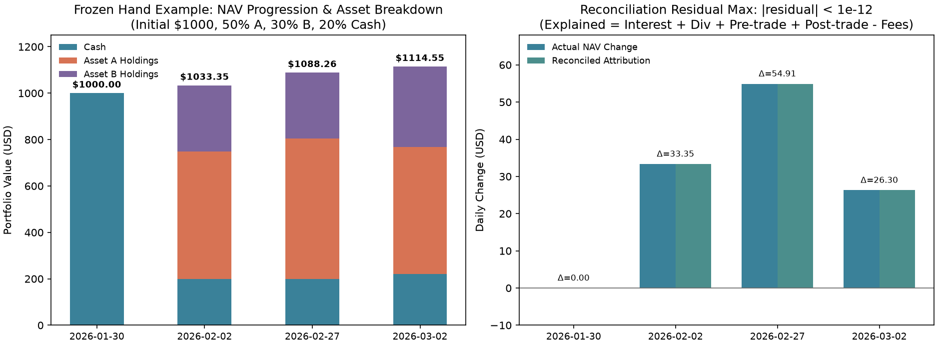
• Left panel (asset composition bars): The x-axis shows dates and the y-axis shows total portfolio assets (USD). It shows how the initial USD 1,000 in cash is converted into assets A and B plus a cash reserve on 2026-02-02; NAV then expands as A rises on 02-27, and the portfolio rebalances successfully on 03-02 to reach USD 1,114.55.
• Right panel (attribution comparison): The x-axis shows dates and the y-axis shows daily NAV changes (USD). Actual NAV changes (dark blue bars) closely match the changes explained by the reconciliation attribution (teal bars); the maximum absolute residual is less than $1.57 \times 10^{-13}$ dollars.
• Key observation: Assets and cash satisfy the self-financing conservation identity at every point, with each flow clearly accounted for.

10.2 Weight Drift and Rebalancing Turnover

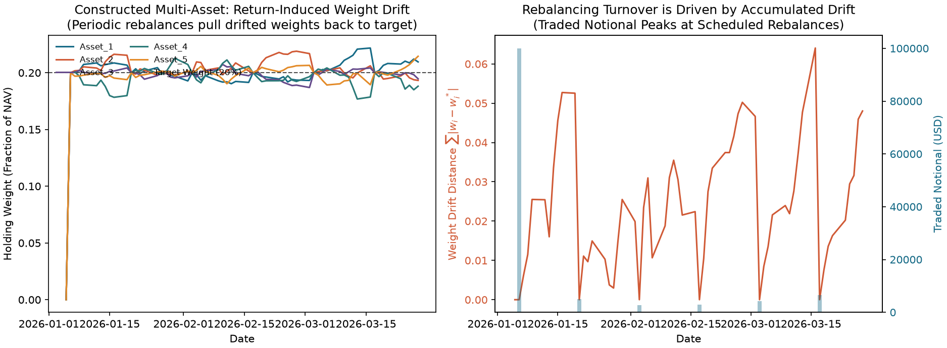
• Left panel (holdings-weight paths): The x-axis shows dates and the y-axis shows portfolio weights. In the constructed market with 5 assets, the target weight is fixed at 20% (black dashed line). The five asset lines in the crowded legend at the left of the original figure are the actual weights of the five assets; the black dashed line represents their common target and is not an additional asset path. The curves retain their historical identity. During each 10-trading-day interval between rebalances, relative asset returns produce a pronounced sawtooth pattern of divergence; weights return to 20% on each rebalancing date.
• Right panel (drift distance and traded notional): The x-axis shows dates. The left axis shows the $L_1$ distance between holdings weights and target weights, $\sum |w_i - w_i^*|$ (orange line); the right axis shows actual traded notional (blue-gray bars).
• Key observation: Rebalancing turnover is a direct consequence of accumulated weight drift. In this fixed constructed setup, larger drift is associated with larger reset trades; cross-sectional dispersion alone is not a general monotonic-turnover theorem.

10.3 Vectorized Backtest Compared with the Event Ledger

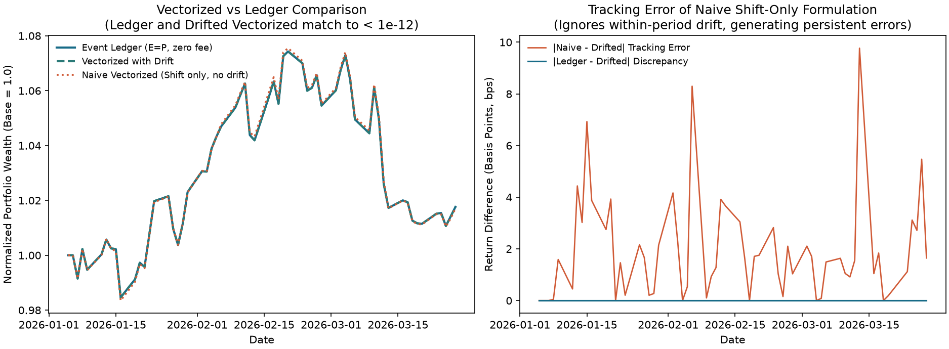
• Left panel (NAV paths): The x-axis shows dates and the y-axis shows normalized NAV. The dark blue line (event ledger with zero fees and closing-price execution) and the green dashed line (vectorized algorithm with weight drift) overlap exactly (difference $< 10^{-15}$); the orange dotted line (naive shift vectorization) diverges visibly.
• Right panel (single-period tracking error): The x-axis shows dates and the y-axis shows return differences (basis points, bps). The dark blue line (difference between the ledger and drift-aware vectorization) is zero to machine precision. The orange line (difference between naive vectorization and actual returns) shows persistent deviations on non-rebalancing dates, with a maximum daily deviation of about 9.77 bps (0.000977).
• Key observation: Vectorized backtests that ignore weight drift have material model bias and cannot replace a ledger based on actual holdings.

10.4 Trading-Cost Sensitivity and Compounding Drag (Kenneth French 10 Industries)

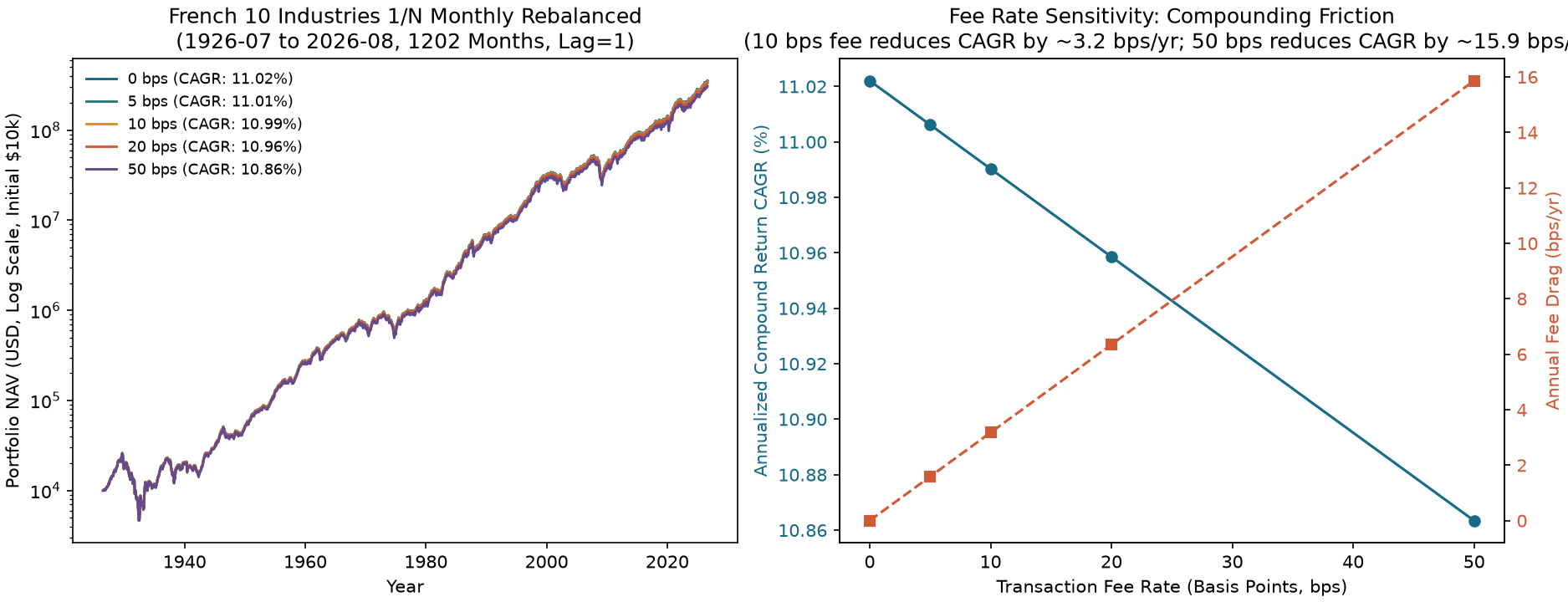
• Left panel (full-sample log NAV curves): The x-axis shows years (1926–2026) and the y-axis shows portfolio NAV on a logarithmic scale (initial value USD 10,000). It shows the divergence in NAV paths under five fee rates: 0 bps, 5 bps, 10 bps, 20 bps, and 50 bps.
• Right panel (annualized CAGR and friction drag; the original title is cut off at the edge, and this gives its full meaning): The x-axis shows the trading fee rate (bps), the left axis shows net annualized compound growth rate (CAGR, %), and the right axis shows annualized performance drag (bps).
• Key observation: As the fee rate rises from 0 bps to 50 bps, the annualized return falls from 11.02% to 10.86% (each 10 bps of fees lowers CAGR by about 3.2 bps per year; a 50 bps fee lowers CAGR by about 15.9 bps per year).

11. A Ledger Case Using Historical Return Proxies

11.1 Historical Data Specification and Sources

This section retains an earlier historical proxy-ledger study. French raw, extracted, and processed data are not bundled in the default I3 reader package; the paths below identify sources in the full project. Data-use rights, subject, and purpose remain unresolved. Public availability is not authorization to redistribute data or execute research. Acceptance of the A10-A limited-scope design and A10-A.1 technical protocol does not replace data rights or execution authorization; G05/A10-B remains unauthorized. Aggregated monthly industry returns are not company-level point-in-time (PIT) inputs. Real membership, tradable prices, corporate actions, borrow/financing, capacity, and trading calendars require separate checks. These curves do not demonstrate deployable market returns. This section reports an empirical analysis using monthly value-weighted returns for the 10 Industry Portfolios published by the Kenneth French Data Library:

• Data file: data/processed/french_10_industries_monthly.csv
• Checksum (SHA-256): 3b097d810c295d64eedfa1ece7067ff2a0707f5ca90e33935df9949251f70950 (the corresponding manifest is data/manifests/french_industries_2026-10-05.json, SHA-256 3b71cd5f781f9790cc380195c22635e03e9c9e27a5f43cd2d0d46fb12efa8271)
• Risk-free rate file: data/processed/french_factors_3_monthly.csv (SHA-256 c19770a19a0ac47ad1c29074f57234570aeaa9725212cb4fa8146a2846c52814).
• Sample period: July 1926 through August 2026 (1,202 calendar months in total).
• Industries: NoDur (consumer nondurables), Durbl (consumer durables), Manuf (manufacturing), Enrgy (energy), HiTec (high technology), Telcm (telecommunications), Shops (retail and wholesale), Hlth (healthcare), Utils (utilities), and Other.
• Conventions and timing:
  1. The data contain only discrete month-end observations. The backtest therefore sets $\text{lag} = 1$: an industry-allocation target calculated at month-end $s$ is filled at the proxy price level at the next month-end, $s+1$ (a full one-month execution lag; the execution price $E$ equals the mark price $P$ at that point).
  2. After adding a base price level of 100 at 1926-06, the first return month, 1926-07, enters at that month-end proxy price, $E=P$. There is no pre-entry equity-price PnL. Its return is zero when $c=0$ and negative from entry fees when $c>0$; holding-period price returns start subsequently. The 1202 return observations include this initial execution month; do not replace them with 1201 months and re-estimate the frozen CAGR.
  3. The number of years used for CAGR is based on the total number of months: $Y = 1202 / 12 \approx 100.167$ years, and $\text{CAGR} = (\text{NAV}_T / \text{NAV}_0)^{12 / 1202} - 1$.
  4. The Sharpe ratio uses aligned monthly Kenneth French FF3 risk-free rates (RF, in decimal form). It is annualized by multiplying the mean monthly excess return divided by its sample standard deviation by $\sqrt{12}$; its statistical properties are discussed in Chapter 32.
  5. The industry total-return index series is a Total-Return Proxy Level. It includes reinvested dividends and is not an individual-stock trading price. The backtest does not add external cash dividends a second time.

11.2 Strategy Design and Backtest Results

The strategy is a simple monthly 1/N rebalancing strategy:

• Decision frequency: Set target weights at each month-end (10% per industry).
• Execution: Execute at the following month-end using $\text{lag} = 1$, with initial cash of USD 10,000.
• Fee rates: $c \in \{0, 5, 10, 20, 50\}$ bps.

Measured Performance Comparison (1926-07 to 2026-08)

Holdings path and performance (same fee-rate experiment):

Trading frictions and realized turnover:

Empirical findings using the historical data:

1. Equivalence check: At 0 bps, the maximum absolute difference between the monthly return series from the ledger and the vectorized output from drifted_weight_returns is $6.52 \times 10^{-16}$, again confirming Theorem 3 at machine precision.
2. Measured drift bias: If rebalancing is changed to once every 12 months (annual rebalancing), the naive shift vectorization that ignores within-year drift reaches a maximum monthly tracking deviation of 2.41% (241 basis points).
3. Cost sensitivity: Average monthly turnover for the 1/N strategy is about 2.38% (about 28.6% annualized). As the fee rate rises from 0 bps to 50 bps, the annualized Sharpe ratio declines gradually from 0.495 to 0.487, CAGR falls by about 15.9 basis points, and ending NAV declines by about USD 47.18 million (about 13.3%).

12. Common Errors

12.1 Error 1: Filling a Closing Signal at the Same Close (Look-Ahead Fill)

• Why it is wrong: If a signal is calculated at the close and filled at that same closing price, the backtest effectively uses the full day's future price movement to trade retroactively.
• Verification code: The backtest engine enforces $\text{lag} \ge 1$ and rejects any zero-lag input that would look ahead.

import pandas as pd
import pytest
from quant_course.backtest import BacktestConfig, run_backtest

dates = pd.date_range("2026-01-05", periods=3, freq="B")
mark = pd.DataFrame({"A": [10.0, 11.0, 12.0]}, index=dates)
tw = pd.DataFrame({"A": [1.0]}, index=[dates[0]])

# The engine raises ValueError when it detects lag=0 (a closing signal filled at the same close)
with pytest.raises(ValueError, match="lag"):
    run_backtest(mark, tw, BacktestConfig(initial_cash=1000.0, lag=0))
print("run_backtest strictly rejects a look-ahead fill with lag=0.")

12.2 Error 2: Using Adjusted Prices and Adding Cash Dividends Again (Double Counting)

• Why it is wrong: A total-return adjusted price already embeds reinvested dividends. Booking cash dividends again counts the return twice. Unadjusted prices must instead be paired with explicitly recorded dividend and split events.
• Verification code:

import numpy as np
import pandas as pd
from quant_course.backtest import BacktestConfig, run_backtest

dates = pd.date_range("2026-01-05", periods=3, freq="B")
mark = pd.DataFrame({"A": [10.0, 10.0, 5.0], "B": [20.0, 20.0, 20.0]}, index=dates)
tw = pd.DataFrame({"A": [1.0], "B": [0.0]}, index=[dates[0]])
cfg = BacktestConfig(initial_cash=100.0)

# Unadjusted prices plus a recorded split preserve the $100 market value
splits = pd.DataFrame({"A": [np.nan, np.nan, 2.0]}, index=dates)
res_split = run_backtest(mark, tw, cfg, splits=splits)
assert np.isclose(res_split.ledger["nav"].iloc[2], 100.0)

# Without the recorded split, NAV incorrectly falls to $50
res_no_split = run_backtest(mark, tw, cfg)
assert np.isclose(res_no_split.ledger["nav"].iloc[2], 50.0)
print("With unadjusted prices, splits must be booked explicitly.")

12.3 Error 3: Replacing Weight Drift with a Simple shift(1) (Naive Vectorized Drift Blindness)

• Why it is wrong: Naive shift vectorization assumes that the portfolio is rebalanced to target weights for free every period, ignoring the weight drift caused by relative asset returns.
• Verification code:

import numpy as np
import pandas as pd
from quant_course.backtest import drifted_weight_returns

# Assume there is no rebalancing for 2 months and both initial weights are 50%
px = pd.DataFrame({"A": [10.0, 20.0, 10.0], "B": [10.0, 10.0, 10.0]}, index=pd.date_range("2026-01-01", periods=3))
tw = pd.DataFrame({"A": [0.5], "B": [0.5]}, index=[pd.Timestamp("2026-01-01")])

# 1. Drift-aware vectorization
r_drift = drifted_weight_returns(px, tw)
# 2. Naive shift vectorization
r_naive = (tw.reindex(px.index).ffill().shift(1).fillna(0) * px.pct_change(fill_method=None).fillna(0)).sum(axis=1)

print("True drifted return at t=2:", round(r_drift.iloc[2], 4))
print("Naive shift return at t=2:", round(r_naive.iloc[2], 4))
assert abs(r_naive.iloc[2] - r_drift.iloc[2]) > 0.08

12.4 Error 4: Ignoring Post-Fee NAV Scaling and Creating a Cash Deficit

• Why it is wrong: If the strategy does not call solve_post_fee_nav to solve for $V'$, and instead trades using $V_{\text{pre}}$, the fees have no funding source and cash becomes negative.
• Verification code:

import numpy as np
from quant_course.backtest import solve_post_fee_nav

v_pre = 1000.0
w = np.array([0.5, 0.5])  # Intended 100% fully invested long exposure
c = 0.002

# Naive, incorrect approach: order at full V_pre and create a negative cash balance
order_val_naive = w * v_pre
fees_naive = c * float(np.abs(order_val_naive).sum())
cash_deficit = v_pre - float(order_val_naive.sum()) - fees_naive
assert cash_deficit < 0  # $2.0 cash overdraft!

# Correct approach: solve for post-fee NAV V' with solve_post_fee_nav
v_post = solve_post_fee_nav(v_pre, np.zeros(2), w, c)
order_val_correct = w * v_post
fees_correct = c * float(np.abs(order_val_correct).sum())
cash_end = v_pre - float(order_val_correct.sum()) - fees_correct
assert np.isclose(cash_end, 0.0)  # Cash is exactly zero; there is no overdraft
print(f"Naive cash deficit: {cash_deficit:.2f}, Post-fee NAV solves exact cash: {cash_end:.4f}")

13. Applications in Quantitative Research

13.1 A Standardized Research Workflow from Strategy Idea to Post-Fee NAV

A sound quantitative research report should apply the following five standard checks before presenting a strategy's NAV:

1. Timing audit: State the signal formation timestamp (signal_time) and execution timestamp (trade_time). The report must establish that available_at $\le$ signal_time $<$ trade_time.

2. Price-type check: A real-share ledger should use unadjusted closing prices in mark_prices and record corporate actions. A synthetic total-return proxy should be declared as using virtual units, without booking dividends twice. If execution uses an opening price or VWAP, provide exec_prices separately.

3. Self-financing reconciliation: Run reconcile and check the relative residual only for positive, finite NAV:

   $$\max_{t:\,0<V_t<\infty} \frac{|\text{residual}_t|}{V_t} \le 10^{-12}$$

   If there are no such periods, the relative check is inapplicable; an empty set is not a pass. Report the absolute currency residual separately for a nonpositive terminal NAV, and investigate nonfinite values. The threshold is an engineering check at the stated scale; also report the maximum absolute error. Passing reconciliation is a necessary check of internal accounting consistency, not sufficient evidence that prices and timestamps are correct. Investigate possible omitted cash flows, double-counted dividends, or split-share mismatches.

4. Tiered cost stress test: Do not report only a zero-fee or single-fee NAV chart. Consider showing the Sharpe ratio and CAGR decay curves under $c \in \{0, 5, 10, 20, 50\}$ bps, and calculate the strategy's break-even fee rate.

5. Falsification and benchmark comparison: Set a benchmark portfolio (such as a 1/N equal-weight buy-and-hold strategy) and test whether the strategy's excess return is merely exposure to overall market beta or passive exposure from unrebalanced drift.

14. Chapter Summary

This chapter establishes the core accounting framework for quantitative textbook Part V. The concepts and rules fit together as follows:

1. Self-financing and the conservation law: In an account with no external cash flows, the change in portfolio NAV follows this accounting identity:

   $$\Delta \text{NAV}_t \equiv \text{Interest}_t + \text{Div}_t + \text{DelistNet}_t + \Delta P_{\text{pre}} + \Delta P_{\text{post}} - \text{Fees}_t$$

   For positive, finite NAV, use Section 6.1’s engineering threshold for the relative residual and report absolute currency errors separately. Exclude nonpositive terminal NAV from that division and investigate nonfinite results. Internal reconciliation does not prove that market data or timestamps are correct.

2. The nonlinear nature of post-fee NAV: Trading costs directly reduce the capital available for allocation. Target holdings must therefore be sized from post-fee NAV, $V'$, by solving the piecewise-linear equation $V' = V_{\text{pre}} - c\sum |w^* V' - x|$. When $c\sum |w^*| < 1$, the real root is globally unique over $\mathbb{R}$; the root lies in $(0, V_{\text{pre}}]$ if and only if $c\sum |x_i| < V_{\text{pre}}$. Starting from $V_{\text{pre}}$, Newton's method has a convex, piecewise-linear objective: its tangent-line zero decreases monotonically and always remains at or above the true root. It terminates in finitely many steps in exact arithmetic; the floating-point implementation uses a relative-residual threshold and a 100-iteration limit.

3. Actual holdings generally drift away from target weights: Target weights hold only momentarily, once a trade completes. Under the assumptions in Section 6.3, without rebalancing weights evolve as $w_{i,t+1} = w_{i,t} \frac{1+r_{i,t+1}}{1+r_{p,t+1}}$; equal returns, zero holdings, or a pure-cash portfolio can remain unchanged. Naive shift vectorization that ignores drift produces returns detached from actual holdings.

4. Causal timing and the execution-lag constraint ($\text{lag} \ge 1$): A signal calculated at the close cannot be filled at that same day's closing price. The intraday event order is fixed: settle interest $\to$ apply corporate actions $\to$ execute at price $E$ $\to$ mark to market at closing price $P$. Invariance to future perturbations is a structural requirement. Existing finite constructed tests cover selected paths; they do not prove invariance to every future change. Complete signals and inputs still require point-in-time contracts and structural reasoning.

5. Building on this chapter: The reconciled ledger, holdings table, and trade blotter produced here become analysis tools in Chapter 30 to expose how 8 common backtest biases distort NAV; in Chapter 31 to construct rigorous time-series splits; in Chapter 32 to calculate rigorous out-of-sample statistical inference; and in Chapter 33 for portfolio risk modeling.

15. Conceptual and Mathematical Questions

• 29-E01: Starting from the beginning- and end-of-period cash and holdings definitions in the self-financing ledger of Section 6.1, write out the complete algebraic derivation including dividends, splits, delistings, pre-trade price changes, post-trade price changes, and trading fees, and prove that the theoretical reconciliation residual is exactly 0.
• 29-E02: Suppose a portfolio starts entirely in cash, with $V_{\text{pre}} = 10,000$ dollars. Its target weights are 0.4, 0.3, and 0.2 in 3 stocks, with 0.1 retained as cash. The proportional trading fee rate is $c = 0.0015$. Use the closed-form solution in Theorem 2 to calculate by hand the post-fee NAV $V'$, total fees payable, purchase amount for each stock, and ending cash balance. Verify that cash as a share of $V'$ is exactly 10%.
• 29-E03: Discuss in detail how the derivative of $f(v) = v + c\sum_i |w_i^* v - x_i| - V_{\text{pre}} = 0$ changes sign when $c \sum_{i=1}^N |w_i^*| \ge 1$. Explain why the function may then lose strict monotonicity and can have multiple roots or no root. Use the counterexample $C=0, x=(1000, -990), V_{\text{pre}}=10, c=0.01$ to explain the economic meaning of a nonpositive root when $c\sum |x_i| \ge V_{\text{pre}}$, and describe the engine's policy response.
• 29-E04: At period $t$, a portfolio holds two stocks with weights $w_{1,t} = 0.6$ and $w_{2,t} = 0.4$, with no cash. Over $[t, t+1]$, stock 1 returns +20% and stock 2 returns -10%. If no trades occur during the interval, calculate the drifted weights of both stocks at the end of period $t+1$.
• 29-E05: Why should a Total Return Index not be used as an unadjusted trading price in an execution module? If a strategy uses total-return prices as input and also passes in a cash-dividend table, how will this distort NAV?
• 29-E06: Explain why the four conditions in Theorem 3 are sufficient, but not necessary, for a vectorized backtest and an event-ledger backtest to match day by day. Give a specific scenario in which the two series remain exactly equal over a particular interval despite a fee rate $c > 0$. Then analyze why a vectorized backtest diverges when $c = 5$ bps and the execution price is the opening price, $E \ne P$.

29-N01: Diagnose Units and Boundaries Along the Ledger Clock (New)

Redo the small ledger in Section 5.2.1. First calculate $C_{\mathrm{pre}},x,V_{\mathrm{pre}},V',\Delta M,\Delta q,C_t,q_t,V_t$, then independently verify it with the conservation decomposition. Identify two errors: writing $0.8V'$ as a share count, and still multiplying the post-trade price P&L by the old 16 shares. Finally explain whether the default $E=P$ means execution at the open, whether monthly-index lag=1 means the next day, and why the recovery value at the same day's close cannot be used after pre-execution NAV falls to or below 0.

16. Programming Questions

Programming Implementation and Boundary-Acceptance Questions

• 29-P01: Write a standalone Python function named solve_nav_closed_form that takes $V_{\text{pre}}$, the vector of current holding values $x$, target weights $w^*$, and fee rate $c$. Assuming the signs of the trade directions are known, use the analytical expression in Theorem 2 to calculate $V'$. Add assertions that numerically compare this function with the Newton solution from solve_post_fee_nav and verify that they agree to machine precision.
• 29-P02: Use run_backtest and reconcile to write an automated test script that fully reproduces the two-asset worked example in Section 8. Assert the share counts, fees, ending cash, ending NAV, and reconciliation residual for all 4 dates. Use an absolute floating-point tolerance of abs=1e-4.
• 29-P03: Write a comparison experiment that generates random price data for 3 assets over 60 trading days. Run drifted_weight_returns and the naive forward-filled expression (tw.shift(1) * ret).sum(axis=1), then calculate and print the maximum return deviation between them on non-rebalancing dates.
• 29-P04: Implement a ruin-termination unit test. Build a leveraged portfolio with a -100% short position in stock X and a +100% long position in stock Y. When a sharp rise in X drives account NAV below zero, assert that the backtest engine triggers termination (terminated_at is not None) and generates no NAV for any later date.

17. Challenge Questions

Advanced Challenges and Further Research

• 29-C01 (No-Trade Bands and Convex Optimization with Proportional Trading Costs): In real-market rebalancing, quantitative funds often use no-trade bands to avoid unnecessary fees from small weight deviations: a trade is triggered only when the actual holding weight is farther from the target than a tolerance $\delta$ (for example, $|w_i - w_i^*| > \delta$), and the holding is adjusted only to the band's boundary. Formulate this mathematically as a one-period utility-maximization problem with an $L_1$ friction penalty, and explain how it corresponds to convex optimization.
• 29-C02 (Complete Ledger Modeling of Short-Borrow Costs and Securities-Lending Interest): This chapter's engine assumes that allow_short=True incurs no additional borrow fee. In real securities lending, a short position incurs a daily borrow cost at an annualized borrow rate $r_{\text{borrow}}$, while short-sale proceeds are usually subject to rehypothecation and collateral and rebate-rate restrictions. Derive the discrete cash and NAV conservation recursions that include borrow costs, and explain how to extend the attribution terms in reconcile accordingly.

18. Complete solutions

29-E01: derive the conservation identity

After a split, $q'_{i,t-1}=q_{i,t-1}S_{i,t}$ and $\widetilde P_{i,t-1}=P_{i,t-1}/S_{i,t}$. The previous value is unchanged: $q'\widetilde P=qP$. Let $I,D,K,L,F$ denote interest, signed dividends, delisting cash, previous value of delisted shares, and trading fees, as in Section 6.1. For live names,

Substitute into the difference of closing NAVs:

All steps are exact rearrangements. Thus actual NAV change minus these components is exactly zero in real arithmetic. Split units and delisting removal are essential to the cancellation; execution-time termination uses $E$ as the final mark and excludes the last segment.

29-E02: buy from cash

All three trades are buys from $x=0$. The stock target sum is $0.4+0.3+0.2=0.9$, leaving cash fraction 0.1. Therefore

Purchases are $3994.6073$, $2995.9555$, and $1997.3036$ in currency units, totaling $8987.8664$. Fees are

Cash is

Using unrounded values, $998.651821/9986.518210=0.1$, exactly the requested cash fraction.

29-E03: the theorem's domain and the financial domain

The function is convex and piecewise linear even outside A3. Away from kinks its derivative is $1+c\sum_iw_i^*\operatorname{sgn}(w_i^*v-x_i)$; at a zero term select any value in $[-1,1]$ for a legal subgradient.

When $c\sum|w_i^*|\ge1$, the far-left slope is $1-c\sum|w_i^*|\le0$ and the far-right slope $1+c\sum|w_i^*|>0$. Slopes are nondecreasing. There may be no root, a single root, two roots, or a flat interval of roots; a convex function cannot repeatedly cross the axis.

• With $x=0,C=V_{\mathrm{pre}}=100,w^*=1,c=2$, $f(v)=v+2|v|-100$ has roots $100/3$ and $-100$. The positive financial root is unique: buy $100/3$ in notional, pay $200/3$ in fees, and retain zero cash. NAV is $100/3$. The negative algebraic root is not a financial candidate.
• With $x=200,C=-100,V_{\mathrm{pre}}=100,w^*=1,c=2$, the minimum of $v+2|v-200|-100$ occurs at $v=200$ and equals 100, so there is no real root.

Failure of A3 removes a sufficient global-monotonicity condition; it does not make every positive-root account impossible. solve_post_fee_nav deliberately rejects inputs outside that supported domain.

Even inside A3, positivity additionally requires $f(0)<0$. For $x=(1000,-990),C=0,V_{\mathrm{pre}}=10,c=0.01$, liquidation fees are $0.01(1990)=19.9$ and $f(0)=9.9>0$. The theorem's unique root is nonpositive, so the engine refuses that rebalance. Equality also fails the positive-equity requirement. This is distinct from a pre-execution ruin, which terminates without trading.

29-E04: compute signed drift

Portfolio return is $0.6(0.2)+0.4(-0.1)=0.08$. Hence

The weights sum to 1. Stock 1 rises by 6.67 percentage points, and stock 2 falls by 6.67 percentage points.

29-E05: do not count dividends twice

A total-return index compounds a dividend-reinvestment convention into its changes. If the engine also receives the corresponding dividend cash table, the same economic benefit enters twice and NAV is overstated.

An index level is not an actual per-share quote. Treating a high accumulated index level as a real quote misstates whole-share and entitlement units. Nevertheless, proportional fees and dollar holdings are invariant to a constant price rescaling with inverse fractional-share scaling. A declared synthetic proxy with no additional dividends is coherent for Section 11's teaching comparison; it does not establish actual security execution.

29-E06: sufficient is not necessary

With aligned initial state, execution dates, and policy, Theorem 3's four conditions make both systems value the same exposure and cash flows at every step. Induction then gives identical returns.

For a counterexample to necessity, consider an interval with no trades, zero cash rate, and $E=P$. A configured positive fee rate, even 10 bps, causes no fee when traded notional is zero. Equality can therefore hold without a zero configured rate.

With actual trading at 5 bps, fees reduce cash and the allocation base; a bare dot product omits them. If $E\ne P$, old shares earn the previous-close-to-$E$ segment and new shares earn $E$-to-close. A single close-to-close return cannot generally allocate both correctly. Thus the simple formula generally fails for the same strategy, but no trade, no holdings, or an offsetting coincidence can still produce equality. Positive fees and unequal price inputs alone do not force a difference at every observation.

29-N01: follow the units through the clock

Interest is $200(0.001)=0.2$; the split creates 16 shares and dividend cash 16. Thus $C_{\mathrm{pre}}=216.2,x=16(49)=784,V_{\mathrm{pre}}=1000.2$. On the buy segment,

The target-dollar change is $\Delta M=0.8V'-784=16.1342>0$, confirming the buy. Divide by 49 to get $\Delta q=0.3293$ shares. Fees are 0.0323; cash is 200.0335; new shares 16.3293; closing NAV 1016.4970.

The independent check is

The quantity $0.8V'$ has dollar units, not share units. Post-trade PnL uses the new shares, not the old 16. Default $E=P$ is a closing-mark proxy, not an open; monthly lag 1 is one monthly observation. Nonpositive execution equity stops at $E$ without later recovery; positive equity with unaffordable costs is rejected; a valid trade followed by nonpositive closing NAV stops at $P$.

29-P01: complete runnable solution

import numpy as np
import pytest
from quant_course.backtest import solve_post_fee_nav


def solve_nav_closed_form(
    v_pre: float, x: np.ndarray, w: np.ndarray, c: float, signs: np.ndarray
) -> float:
    """Post-fee NAV from Theorem 2, conditional on consistent trade signs."""
    numerator = v_pre + c * float(np.sum(signs * x))
    denominator = 1.0 + c * float(np.sum(signs * w))
    return numerator / denominator


# Compare the closed form and the existing solver.
v_pre = 1000.0
x = np.array([400.0, 500.0])
w = np.array([0.6, 0.2])
c = 0.01

# Try a buy in asset 1 and a sale in asset 2; verify signs after solving.
signs = np.array([1.0, -1.0])

v_closed = solve_nav_closed_form(v_pre, x, w, c, signs)
v_newton = solve_post_fee_nav(v_pre, x, w, c)

print(f"Closed-form V': {v_closed:.6f}")
print(f"Newton solver V': {v_newton:.6f}")
assert np.isclose(v_closed, v_newton, rtol=0, atol=1e-10)
assert np.array_equal(np.sign(w * v_closed - x), signs)
print("P01 verification passed successfully!")

29-P02: complete runnable solution

import numpy as np
import pandas as pd
import pytest
from quant_course.backtest import BacktestConfig, reconcile, run_backtest

dates = pd.DatetimeIndex(["2026-01-30", "2026-02-02", "2026-02-27", "2026-03-02"])
mark = pd.DataFrame(
    {"A": [10.0, 11.0, 12.1, 12.0], "B": [20.0, 19.0, 19.0, 21.0]},
    index=dates,
)
execp = pd.DataFrame(
    {"A": [10.0, 10.0, 12.0, 12.0], "B": [20.0, 20.0, 19.5, 20.0]},
    index=dates,
)
tw = pd.DataFrame({"A": [0.5, 0.5], "B": [0.3, 0.3]}, index=[dates[0], dates[2]])
cfg = BacktestConfig(initial_cash=1000.0, fee_rate=0.002, lag=1)

res = run_backtest(mark, tw, cfg, exec_prices=execp)
led = res.ledger
rec = reconcile(res, mark, cfg, exec_prices=execp)

# Complete four-date state: q_A, q_B, cash_end, fees, nav.
# Independently computed closed-form expectations; rtol=0 fixes absolute tolerance.
expected = np.array([
    [0.0, 0.0, 1000.0, 0.0, 1000.0],
    [49.920128, 14.976038, 199.680511, 1.597444, 1033.346645],
    [49.920128, 14.976038, 199.680511, 0.0, 1088.258786],
    [45.753458, 16.471245, 219.616601, 0.159808, 1114.554248],
])
actual = np.column_stack([
    res.positions[["A", "B"]].to_numpy(),
    led[["cash_end", "fees", "nav"]].to_numpy(),
])
assert led.index.equals(dates)
np.testing.assert_allclose(actual, expected, rtol=0, atol=1e-4)
assert rec["residual"].abs().max() < 1e-12
assert rec["cash_identity"].abs().max() < 1e-12
print("P02: all four dates, both positions, cash, fees, NAV and reconciliation checked.")

The five columns cover both share counts, cash, fees, and NAV on every input date. Absolute tolerance is $10^{-4}$ with relative tolerance disabled. Reconciliation and the cash identity are checked independently to $10^{-12}$.

29-P03: complete runnable solution

import numpy as np
import pandas as pd
from quant_course.backtest import drifted_weight_returns

rng = np.random.default_rng(2026)
dates = pd.date_range("2026-01-01", periods=60, freq="B")
shocks = rng.normal(0, 0.02, size=(60, 3))
px = pd.DataFrame(100.0 * np.exp(np.cumsum(shocks, axis=0)), index=dates)

# Form equal-weight signals every 20 observations; delay execution by one row.
sig_dates = dates[[0, 20, 40]]
tw = pd.DataFrame(1.0 / 3.0, index=sig_dates, columns=px.columns)

trade_w = tw.copy()
trade_w.index = dates[np.searchsorted(dates, tw.index) + 1]

r_drift = drifted_weight_returns(px, trade_w)
r_naive = (
    trade_w.reindex(dates).ffill().shift(1).fillna(0)
    * px.pct_change(fill_method=None).fillna(0)
).sum(axis=1)

non_trade = ~dates.isin(trade_w.index)
max_error = np.abs(r_naive[non_trade] - r_drift[non_trade]).max()
print(f"Max tracking error between naive shift and drifted: {max_error:.6f}")
assert max_error > 1e-4
print("P03 passed: naive shift-only formulation diverges as predicted!")

29-P04: complete runnable solution

import pandas as pd
import pytest
from quant_course.backtest import BacktestConfig, run_backtest

dates = pd.date_range("2026-01-05", periods=4, freq="B")
# X jumps from 10 to 25 after the short is established.
mark = pd.DataFrame(
    {"X": [10.0, 10.0, 25.0, 30.0], "Y": [20.0, 20.0, 20.0, 20.0]}, index=dates
)
# Short X and go long Y.
tw = pd.DataFrame({"X": [-1.0], "Y": [1.0]}, index=[dates[0]])
cfg = BacktestConfig(
    initial_cash=100.0, allow_short=True, max_gross=2.0, lag=1
)

res = run_backtest(mark, tw, cfg)

print("Terminated at:", res.terminated_at)
print("Ledger length:", len(res.ledger))
print("Final NAV:", res.ledger["nav"].iloc[-1])

assert res.terminated_at == dates[2]
assert len(res.ledger) == 3
assert res.ledger["nav"].iloc[-1] <= 0.0
print("P04 passed: ruin policy correctly terminated bankrupted backtest!")

29-C01: the static no-trade region

Let $u$ be current drifted weights, $w$ the chosen new weights, $\mu$ expected returns, $\gamma>0$ risk aversion, $\Sigma\succ0$ the covariance matrix, and $c>0$ the cost coefficient. With no further investment constraints, consider the static approximation

Strict concavity gives a unique optimum. The subgradient optimality condition is

At $w=u$, every absolute-value subgradient coordinate can take any value in $[-1,1]$. Thus no trade is optimal if and only if

This is a region of current states $u$, not a fixed box that must contain all optimal weights. With frictionless optimum $w^0=(\gamma\Sigma)^{-1}\mu$,

Positive definiteness makes $\gamma\Sigma$ invertible. The region is therefore a bounded closed convex parallelotope centered at $w^0$. It is generally tilted with correlated assets and axis-aligned when $\Sigma$ is diagonal. A merely positive-semidefinite matrix can have a nullspace that makes the region unbounded; the bounded-parallelotope claim would fail.

Outside this region solve the same subgradient equation. A traded coordinate satisfies $\mu_i-(\gamma\Sigma w)_i=c\operatorname{sgn}(w_i-u_i)$; an unchanged coordinate has marginal benefit within $[-c,c]$. The kink can therefore leave coordinates exactly unchanged. “Trade to the boundary” here means that remaining marginal benefit reaches marginal cost in this static model. It is not a proof that every hand-chosen threshold $\delta$ is dynamically optimal. The $L_1$ weight difference approximates costs and does not simultaneously solve Section 6.2's exact fee-adjusted denominator. A dynamic policy needs future utility and state transitions.

Assessment: objective and conditions 40%; subgradients and kinks 30%; state-space geometry and limitations 30%.

29-C02: free cash, collateral, and short costs

This is a teaching extension beyond the base engine; allow_short=True does not implement margin accounting. First specify a convention. During a fixed-holding interval assume no new trades, splits, or delistings. Let $q_i$ be signed shares, $F$ free cash, and $R$ restricted collateral. Then

Positive free cash earns $r_l$, negative free cash pays $r_b$, and collateral earns $r_R$. Use the example's declared day-count fraction $h=\Delta d/360$; this is not a universal market rule. Define