Algorithmic Execution and Trade Scheduling

Existing engineering evidence is cited under its original acceptance identity. Main thread: convert portfolio target weights into signed parent orders, balance market impact against execution risk on a discrete execution clock, and attribute and benchmark execution quality ex post through an implementation shortfall decomposition. Prerequisites: Chapter 9, Optimization Foundations; Chapter 34, Market Microstructure; and Chapter 35, Transaction Costs and Capacity. After reading, you should be able to schedule TWAP, forecast-volume VWAP, and POV orders; compute the implementation shortfall decomposition with partial and unfilled quantities; derive the discrete Almgren–Chriss mean-variance objective; and reconcile cash and holdings under a causal clock.

1. Learning Objectives

After completing this chapter, you should be able to:

1. Distinguish four execution benchmarks—Decision Price, Arrival Price, Ex-Post Market VWAP, and Terminal Mark Price—and explain their evaluation settings and economic meanings.
2. Construct discrete child-order schedules for a signed parent order using Time-Weighted Average Price (TWAP), forecast-volume weighting (Forecast-Volume VWAP), and lagged observed volume participation (POV).
3. Distinguish decision, send, arrival, fill, marking, and portfolio-signal times, and explain why monthly signal weights must not be presented as intraday microstructure signals.
4. Compute signed implementation shortfall (IS), decompose it exactly into delay cost, execution cost, unfilled opportunity cost, and explicit fees, and prove its algebraic identity with the direct monetary comparison of paper and actual portfolios.
5. Handle partial-fill and no-fill boundaries. When there are no fills, mark fill VWAP as undefined (NaN/None) to avoid division by zero or misreporting the average as zero.
6. Explain the microstructure difference between temporary and permanent price impact, derive the efficient execution frontier under the discrete-time Almgren–Chriss mean-variance objective, and identify its assumptions and limits.
7. Reconcile changes in cash, holdings, and net asset value (NAV) after actual fills, without charging cash a second time for price impact already embedded in the fill price.

2. Why Quant Needs This

A strategy constructed on paper may show an excellent Sharpe ratio. Once its orders reach a real market, that paper profit can quickly erode. If a trader sends a market order for tens of thousands of shares, the order can sweep through the shallow top levels of the book and incur substantial temporary market impact. If the trader avoids impact by spreading the order over several days, the price may drift upward with the asset, making later shares more expensive and potentially leaving the target position incomplete at the end of the window.

Unfilled quantity affects execution quality relative to the paper target. Suppose a strategy plans to buy an order but the execution algorithm fills only 20%, after which the price rises. The potential gain on the remaining 80%, measured against the arrival-price benchmark, enters IS as opportunity cost. This is a performance-attribution item, not an actual cash-book expense.

Chapters 14–15 established expected asset returns and factor pricing. Chapter 29 built the portfolio backtest ledger and converted weight changes into target share counts. Chapter 34 introduced visible limit-order-book depth, quoted spreads, and queue priority. Chapter 35 quantified spreads, commissions, borrow costs, and impact functions. This chapter handles the implementation stage of the trading pipeline: it takes the target from Chapters 29 and 35, shows how to distribute the total demand over discrete execution windows, and attributes execution quality after trading. The goal of an execution algorithm is not to predict future returns. It is to balance market-impact cost, which tends to increase with trading speed, against execution risk, as prices drift while execution takes longer.

3. Intuition

Consider a simple scenario. At 09:28, you decide to buy 10,000 shares of a stock whose midpoint is USD 100.00. The order reaches the venue at the 09:30 open, when the price has moved to USD 100.20. You must complete the trade between 09:30 and 10:30.

You face two extremes:

• Extreme 1: At 09:30, submit all 10,000 shares as one market order. Visible depth on the first five ask levels is limited, so your buy order consumes them immediately and pushes the average fill price to USD 101.50. You incur substantial temporary impact, but eliminate the risk that the stock continues to rise during the next hour.
• Extreme 2: Split the 10,000 shares into 60 child orders of about 167 shares per minute. Each child order is only a small fraction of that minute's volume, so the book barely notices you and temporary impact is small. However, if external buying pressure moves the price from USD 100.20 to USD 102.00 during the hour, later child orders become increasingly expensive and the final average fill price may reach USD 101.10. Moreover, if 2,000 shares remain unfilled at 10:30 and must be canceled, you miss all of the gains from a subsequent surge in those shares.

Execution algorithms operate between these extremes:

• TWAP divides the parent order evenly across time slots. It suits assets with relatively uniform liquidity or cases without a volume forecast.
• Forecast VWAP allocates the parent order according to a volume curve frozen before trading. If the forecast curve is heavier around the open and close, the schedule assigns more shares to those intervals.
• POV sets the pace of subsequent requests from the chosen denominator convention and the latest fully observed market volume. Actual fills remain subject to current liquidity and capacity.

Implementation shortfall is the final scorecard. It starts its ledger when you decide to trade and decomposes the result into delay loss between the decision and order submission, slippage on actual fills, missed gains or losses on unfilled quantity, and explicit commissions paid to the broker.

4. Mathematical Foundations

Let $Q$ be the signed parent-order quantity for an asset in the portfolio (shares; $Q>0$ for a buy and $Q<0$ for a sell). Divide the execution window into $N$ discrete time slots indexed by $k\in\{1,2,\dots,N\}$, each of length $\Delta t$.

Variables and Notation

• $t_d$: timestamp when the portfolio manager makes the rebalance decision; it maps to the interface field decision_time and benchmark price $P_{\text{decision}}$ (USD/share).

• $t_p$: timestamp when the algorithm receives the parent order; it maps to parent_received_at and satisfies $t_d\le t_p$.

• $t_{\text{arrival}}$: arrival-benchmark time used for IS; it maps to arrival_time and price $P_{\text{arrival}}$ (USD/share). This is an attribution benchmark and must not be conflated with child-order send time or venue-arrival time.

• For each child order $k$, interface fields child_send_at, child_venue_arrival_at, and fill_at map respectively to $t_{\text{send},k}$, $t_{\text{venue},k}$, and $t_{\text{fill},k}$. Fields observed_available_at and forecast_frozen_at record when volume data became available and when the forecast was frozen. The slot-end market mark becomes available only at slot_end and is recorded in slot_mark_available_at. Even when there is no fill, first settle the interval using the old mark, then apply the slot-end mark. The terminal mark time is $t_{\text{terminal}}$, mapped to terminal_mark_time.

• $t_k$: start time of execution slot $k$.

• $q_k$: signed child-order quantity requested in slot $k$ (shares), with the same sign as $Q$.

• $F_k$: signed shares actually matched in slot $k$, satisfying $|F_k|\le |q_k|$. If nonzero, its direction matches $q_k$ and $Q$. This chapter considers a single parent order in one direction, so $\sum_k|F_k|=|F|$; this identity must not be generalized to mixed buys and sells.

• $P_{\text{fill},k}$: average fill price in slot $k$ (USD/share). It is undefined when $F_k=0$.

• $F$: cumulative signed shares filled over the execution window:

  $$F=\sum_{k\in\mathcal F}F_k$$

• $R$: signed shares remaining unfilled and canceled at the end of the execution window (the remainder, in shares), satisfying the conservation identity:

  $$Q=F+R$$

• $t_{\text{terminal}}$: execution-window end and terminal-mark timestamp. The corresponding terminal mark is $P_{\text{terminal}}$ (USD/share).

• $V_k^{\text{forecast}}$: forecast external-market volume for slot $k$, frozen before the window begins (shares).

• $V_{k-1}^{\text{obs}}$: actual external-market volume in slot $k-1$, fully completed and observed before child order $k$ is sent (shares).

• $V_k^{\text{realized}}$: actual external-market volume during slot $k$ (shares). This is still in the future at time $t_k$ and must not be used to decide the child order.

• $c_{\text{comm}}$: explicit commission rate per share (USD/share). Total explicit fees are $C_{\text{fees}}=|F|\,c_{\text{comm}}$.

From the Ledger to Execution Evaluation: Continue the Same 100-Share Example

Chapter 34's quotes do not determine actual fills; Chapter 35 books only 60 shares and USD 0.30 in fees. After the window closes, Chapter 36 checks IS using $Q=100,F=60,R=40$: $2.00+1.80+3.20+0.30=7.30$. The direct method gives $60(10.05-10.00)+40(10.10-10.00)+0.30=7.30$. This equals paper NAV minus actual NAV and does not change cash of USD 1,396.70 or the actual holding of 60 shares. If windows overlap, before sending a new child order subtract already-sent but unconfirmed quantity from the unfinished parent-order capacity. $R=40$ is the terminal remainder; during execution, do not treat all unconfirmed requests as capacity available for resending.

Now consider selling 100 shares, with only 60 filled, decision price 10.00, arrival price 9.98, fill price 9.95, and terminal price 9.90. Then $Q=-100,F=-60,R=-40$, and the four components remain $2.00,1.80,3.20,0.30$. An account initially holding 100 shares and USD 1,000 in cash ends with USD 1,596.70 in cash and 40 shares, for terminal NAV of USD 1,992.70. The ideal account that sold all 100 shares at the decision price has NAV of USD 2,000; the difference is USD 7.30. Direction follows from signed quantities, not from forcing sell-price differences to be absolute values.

Price Process and Market-Impact Assumptions

In this discrete linear-impact teaching specification, the exogenous price increment unaffected by trading follows arithmetic Brownian motion. After adding contemporaneous permanent impact to the midpoint, the price recursion for signed fills under this chapter's buy-positive, sell-negative convention is:

where:

• $S_k$ is the constructed midpoint at the end of period $k$, including prior permanent impact (USD/share); it is not an observable “true fundamental price.”
• $\sigma$ is the price-diffusion coefficient. If time is measured in days, $\sigma\sqrt{1\text{ day}}$ is the standard deviation of the one-day price increment. Dividing by a locally constant reference price gives the corresponding daily return volatility in Chapter 35. Its units are USD / (share $\cdot$ time$^{1/2}$).
• $\xi_k\sim\mathcal N(0,1)$ are independent standard-normal shocks.
• $F_k$ is signed fill quantity in period $k$; buys are positive and sells negative. For a sell liquidation, $F_k=-n_k$, so the permanent-impact term is $-\gamma n_k$.
• $\gamma$ is the permanent market-impact coefficient (USD/share$^2$); permanent impact enters subsequent midpoint prices.

Within each slot, the fill uses $S_{k-1}$ as its reference, with temporary impact applied to the fill price; noise and permanent price updates occur afterward. Thus the final noise arrives after liquidation. The zero execution variance for $N=1$ follows from this model's timing. Arithmetic Brownian prices do not guarantee positivity over every path, which must not be confused with the positive-price input domain of an engineering implementation.

The actual fill price includes temporary market impact:

where $\eta$ is the temporary-impact coefficient (USD·time/share$^2$). Temporary impact affects only the current fill and does not enter later-slot price updates.

5. Formal Definitions

5.1 Execution Clock and Causal Ordering

In a quantitative trading system, execution, observation, and matching span several clocks. The system must record the signal-freeze time $t_{\text{signal}}$, the decision time $t_d$ when target shares are locked, parent-order receipt time $t_{\text{parent}}$, each child-order send time $t_{\text{send},k}$, venue-arrival time $t_{\text{venue},k}$, fill-report time $t_{\text{fill},k}$, the time POV external volume becomes available to the algorithm $t_{\text{obs},k}$, forecast-freeze time $t_{\text{forecast},k}$, and cancellation and terminal-mark time $t_{\text{terminal}}$. Also record the arrival benchmark time $t_{\text{arrival}}$ and price $P_{\text{arrival}}$ used by IS. In this teaching interface it is the agreed parent-order arrival benchmark; it does not replace any child-order send or venue-arrival time.

The timestamps must satisfy these causal constraints:

arrival_time is only the IS benchmark anchor; it does not mean that the algorithm received the parent order or that a child order arrived at the venue. Slot windows may overlap, and the engine processes slots by index while enforcing nondecreasing child send times. Before each send, the algorithm counts only fills strictly earlier than that send and reserves sent-but-unconfirmed quantities against the parent-order remainder. A send at the same timestamp as a fill confirmation occurs first, so that simultaneous fill cannot affect sizing for that send. POV observations must satisfy observed_available_at <= child_send_at, and the forecast curve must be frozen before the first child order is sent. The current simulation uses zero transmission delay, so child_send_at == child_venue_arrival_at. These are enforceable causal-clock constraints; a later child order need not wait for the previous slot to end.

A monthly rebalance signal represents target holdings derived from monthly financial or low-frequency market data and remains frozen throughout the execution day. The algorithm must not disguise a monthly signal as intraday high-frequency alpha or feed future monthly closing data backward into the intraday execution algorithm.

5.2 Time-Weighted Average Price (TWAP)

TWAP distributes the parent order evenly across $N$ time slots fixed in advance.

The planned child quantity in slot $k$ is:

Conditions:

1. Fix the total execution window $[t_0,t_{\text{terminal}}]$ and the number of slots $N$ before trading begins.
2. Do not dynamically add to or reduce parent order $Q$ during the window.

5.3 Forecast-Volume VWAP Schedule

A VWAP schedule aims to match the shape of child orders to the market's expected intraday volume curve.

Let $V_k^{\text{forecast}}>0$ be the forecast external-market volume in each slot, set before the window begins. The forecast-volume share is:

The planned child quantity in slot $k$ is:

Conditions:

1. The weight vector $\boldsymbol w=(w_1,\dots,w_N)^\top$ must depend only on historical statistics (for example, the median volume in each slot over the previous 20 trading days) and must be frozen completely at $t_0$.
2. The schedule must not use future realized external volume $V_k^{\text{realized}}$ from the current trading day as an input.

The expressions above, like $q_k$ in Section 5.2, define an ex-ante planned curve. When actual volume is insufficient, this chapter's execute_order mechanically reallocates unfilled quantity across later slots based on the current parent remainder. This capacity-constrained catch-up rule does not read future volume and is not an adaptive schedule that updates price or total-volume forecasts from intraday information.

5.4 Ex-Post Market VWAP Benchmark

Ex-post market VWAP is a public external benchmark price used to evaluate institutional execution quality after the whole window has ended:

Here, $P_k^{\text{mkt}}$ and $V_k^{\text{realized}}$ are the average price and volume of the external market in slot $k$, excluding the institution's own fills. If a benchmark including own fills is used instead, its inclusion rule must be stated separately. This benchmark can be computed only ex post; it is not an input to the ex-ante schedule.

5.5 Lagged-Observed Percentage of Volume (POV)

POV, also called a participation-rate algorithm, is reactive. Instead of specifying a complete fixed allocation in advance, it sets target order pace from available liquidity information under a chosen denominator convention. Actual participation remains subject to fills, cancellations, and capacity.

Under a strict causal clock, the algorithm does not know future realized external volume $V_k^{\text{realized}}$ in the current slot when it sends child order $k$ at the slot start. Thus the child quantity can be computed only from $V_{k-1}^{\text{obs}}$, the latest fully settled and observed prior-slot volume.

For a participation rate $\rho\in(0,1)$, two denominator conventions are in use:

The following participation-rate equations first define an uncapped reference request. After the minimum with the remainder is applied, the actual request may fall below that participation rate; actual fills are also constrained by current-slot capacity.

Definition A (exclusive denominator, external-market volume only):

For a nonoverlapping hand calculation, assume prior fills have all been confirmed before the next send and no orders are in flight; only then can one write $Q_{\mathrm{rem},k}=Q-\sum_{j<k}F_j$. In general, send capacity must subtract both already confirmed fills and same-direction quantities still reserved in flight. Do not infer availability merely from slot indices.

Definition B (inclusive denominator, including own fills):

The child quantity is therefore:

Boundary and validity conditions:

1. First-slot boundary: At the first open-market slot, $k=1$, no prior continuous-trading volume is yet observable, so $V_0^{\text{obs}}=0$. Under the contract, POV sends zero in the first slot and waits until that slot's volume has settled before following the market.
2. Limit test: Definition B has a finite solution only for $0\le\rho<1$. As $\rho\to1$ with positive external volume, the uncapped inverse formula diverges; after capping at the finite remaining order, the actual request remains finite. Implementations often also cap requests by remaining quantity, a participation-policy ceiling, and market capacity. A ceiling such as 0.5 is an implementation choice, not a universal threshold implied by the identity.

5.6 Implementation Shortfall (IS)

Perold (1988) is retained here as further reading; the historical check covered author and publisher metadata, without reading the full text. The SEC (2003) discusses cost measurement through the difference between paper and actual portfolios and traces an early source of the idea to Treynor (1981). That request for comments supplies conceptual background, rather than prescribing this chapter's formula. The decomposition below is an explicit teaching convention, not a claim of a single industry-standard method.

For signed parent order $Q$, let the actual fill sequence be $\{(F_k,P_{\text{fill},k})\}_{k=1}^N$, cumulative filled quantity be $F=\sum_kF_k$, and unfilled remainder be $R=Q-F$. Define total implementation shortfall as:

Its components are:

1. Delay cost (slippage from decision):

   $$\text{IS}_{\text{delay}}=Q(P_{\text{arrival}}-P_{\text{decision}})$$

   This measures losses from adverse price movement between the portfolio manager's decision and the order's arrival at the market.

2. Execution slippage cost:

   $$\text{IS}_{\text{exec}}=\sum_{k\in\mathcal F}F_k(P_{\text{fill},k}-P_{\text{arrival}})$$

   When $F\ne0$, if fill VWAP is defined as $P_{\text{fillVWAP}}=\frac{\sum_{k\in\mathcal F}F_kP_{\text{fill},k}}{F}$, then execution cost can also be written as:

   $$\text{IS}_{\text{exec}}=F(P_{\text{fillVWAP}}-P_{\text{arrival}})$$

   This measures slippage of actual fills relative to the arrival benchmark.

3. Unfilled opportunity cost:

   $$\text{IS}_{\text{opp}}=R(P_{\text{terminal}}-P_{\text{arrival}})$$

   This measures potential mark-to-market gains or losses missed because the remainder $R$ was not traded by the deadline.

4. Explicit fees:

   $$C_{\text{fees}}=\sum_{k\in\mathcal F}|F_k|c_{\text{comm}}=|F|c_{\text{comm}}$$

   These are explicit commissions and taxes paid to the broker or venue.

By convention, $\text{IS}>0$ means positive execution cost: actual account NAV is below the frictionless paper portfolio's NAV.

6. Derivations

6.1 Algebraic Proof of the Two Equivalent Representations of IS

In practice, implementation shortfall can be computed in two ways:

1. A four-component decomposition aligned with the workflow: delay, execution, opportunity, and explicit fees.
2. The direct amount method, which directly compares the terminal value of the theoretical paper portfolio with the actual execution cash ledger.

Theorem. The four-component decomposition is algebraically identical to the direct amount method.

Proof. Under the direct amount method, the frictionless paper portfolio is assumed to buy all $Q$ shares at $P_{\text{decision}}$ at the decision time $t_d$. At the terminal time $t_{\text{terminal}}$, the paper position's market value is $Q P_{\text{terminal}}$. It initially spent $Q P_{\text{decision}}$, so its theoretical book profit is:

In actual execution, we buy $F_k$ shares in each slot at $P_{\text{fill},k}$ and pay fees $C_{\text{fees}}$. At the terminal time, the $F$ shares held are marked at $P_{\text{terminal}}$. The actual economic profit is:

Define implementation shortfall as the difference between paper and actual profit:

Substituting the profit expressions gives:

Using quantity conservation, $Q=F+R$, expand $Q P_{\text{terminal}}$ as $(F+R)P_{\text{terminal}}$:

Cancel the $F P_{\text{terminal}}$ terms:

Since $\sum_{k\in\mathcal F}F_k=F$ and $Q=F+R$, decompose $Q P_{\text{decision}}$ as $F P_{\text{decision}}+R P_{\text{decision}}=\sum_{k\in\mathcal F}F_kP_{\text{decision}}+R P_{\text{decision}}$:

This is the classic direct amount formula.

To prove its identity with the four-component decomposition, insert the arrival price $P_{\text{arrival}}$ into each price difference above. For filled quantity:

For unfilled quantity:

Substituting both expansions into the direct amount formula:

Collect the common factor $(P_{\text{arrival}}-P_{\text{decision}})$:

Rearranging the terms:

This proves the result.

The proof shows the sign symmetry: the signed formulas are self-consistent for either a buy ($Q>0$) or a sell ($Q<0$). If a buy faces rising prices, the price difference is positive and IS rises. If a sell faces falling prices, $P_{\text{fill}}-P_{\text{arrival}}<0$ while $F_k<0$, so the product is positive and IS likewise records the loss from a lower sale price.

Other papers or trading systems may allocate the decision-to-arrival price move across filled quantity or use a different opportunity-cost benchmark. This chapter assigns the full $Q$-share decision-to-arrival move to delay cost and measures fills and remainder from arrival price. The components can be allocated differently, but as long as each item is settled consistently against the same decision and terminal prices, the direct-amount total is fixed by the identity.

6.2 Deriving the Discrete Almgren–Chriss Execution Cost–Risk Frontier

Consider liquidating an initial position of $X>0$ shares (a sell order) over total time $T=N\Delta t$. Let $x_k$ be the remaining inventory at timestamp $t_k$, the end of time slot $k$, with boundary conditions:

The number of shares sold in slot $k$ is $n_k=x_{k-1}-x_k\ge0$. This section fixes a deterministic static schedule at the outset; $n_k$ and $x_k$ are nonrandom. The expectation and variance derivations below do not directly apply to inventory that adapts to noise.

From the price process in Section 4:

The fill price includes temporary impact:

Total liquidation proceeds are $W=\sum_{k=1}^N n_k\tilde S_k$. Relative to the initial arrival value $X S_0$, implementation shortfall, excluding explicit commissions, is the random variable:

Step 1: Derive expected shortfall $E[x]$. Expand the fundamental price recursion:

Substitute into the fill-price expression:

Total proceeds are:

Since $\sum_{k=1}^Nn_k=X$ and $E[\xi_j]=0$, expected proceeds are:

Use the discrete-sum identity:

Substituting this into expected shortfall gives:

This section assumes $\eta/\Delta t>\gamma/2$. This is a model condition for a strictly convex objective and the unique solution below, not a universal market fact. Define the adjusted temporary-impact parameter $\tilde\eta=\frac{\eta}{\Delta t}-\frac12\gamma>0$. Expected execution cost is then:

The discrete identity regroups total cost as a constant and a path-dependent term:

The term $\gamma X^2/2$ is the path-invariant constant after this regrouping; it is not the original discrete permanent-impact loss. The original permanent-impact term

still depends on the schedule. Its $-\gamma\sum_kn_k^2/2$ component combines with temporary impact to form $\tilde\eta=\eta/(\Delta t)-\gamma/2$.

Numerical check: let $\gamma=0.01$, $\eta/\Delta t=0.02$, and $X=1{,}000$. For schedule $[1{,}000,0]$, the original permanent term is $0$; for $[500,500]$, it is $0.01\times500\times500=2{,}500$. The regrouped constant $\gamma X^2/2=5{,}000$ is the same for both paths; the path difference appears through the adjusted temporary-impact squared term.

Here $x_t$ denotes remaining inventory decreasing from $X$ to $0$. For the sell schedule, with cumulative sales $y_t=X-x_t$, the permanent-impact cost rate is $\gamma y_t\dot y_t$, whose total is

Using fixed endpoints $x_0=X,x_T=0$, the same total integral can also be written

This is an integral identity after evaluating the boundary terms; the integrands are not equal at each instant. In Challenge 36-C01, $x_t$ instead denotes cumulative buy progress from $0$ to $X$, so the buy-cost rate $\gamma x_t\dot x_t$ integrates with a positive sign.

Step 2: Derive shortfall variance $V[x]$. All uncertainty in shortfall comes from the Brownian-motion term

Reverse the order of summation:

because the $\xi_j$ are independent with unit variance. Thus:

Execution variance is therefore the accumulated squared remaining inventory over time: a larger position held for longer carries more price risk.

Step 3: Solve the optimization problem. Expected shortfall is measured in USD, while variance is measured in USD$^2$. The risk-aversion parameter $\lambda_{\text{risk}}$ must therefore have units USD$^{-1}$ so the terms can be added. It is distinct from the linear impact slope $\lambda_{\text{impact}}$ (USD/share$^2$) in Chapter 35. The time-slot duration $\Delta t$ has units of time; it is not dimensionless turnover $\tau_{\text{turnover}}$. For trader risk aversion $\lambda_{\text{risk}}\ge0$, form the mean-variance objective:

For any intermediate state $x_k$ ($1\le k\le N-1$), the first-order condition is:

Divide by $2\tilde\eta$ and rearrange into a second-order linear difference equation with constant coefficients:

The characteristic equation is $r^2-2\cosh(\kappa\Delta t)r+1=0$, where $\kappa$ satisfies

Here the inventory nodes use $t_k=k\Delta t$, elapsed time from the start, unlike the slot-start times in Section 4. The units of $\kappa$ are time$^{-1}$, making $\kappa\Delta t$ dimensionless. With boundary conditions $x_0=X$ and $x_N=0$, the unique analytic solution of the difference equation is:

Special cases. When $\lambda_{\text{risk}}=0$ or $\sigma=0$, $\kappa=0$ and the continuous limit applies. By L'Hôpital's rule:

Then $n_k=x_{k-1}-x_k=X/N$, so the optimal liquidation path degenerates to strictly linear liquidation, or TWAP.

When $\lambda_{\text{risk}}>0$ and $\sigma>0$, before maturity the hyperbolic-sine curve gives a decreasing, convex remaining-inventory path ($x''(t)=\kappa^2x(t)>0$). The trader sells faster early (front-loads execution), accepting higher temporary impact in exchange for quickly reducing exposure and lowering variance.

7. Financial Interpretation

7.1 Agency and the Choice of Benchmark

The benchmark chosen for an execution algorithm directly affects the trader's incentives:

1. Arrival Price: When an order is meant to stay close to the price at the agreed post-decision arrival point, arrival price can evaluate delay and subsequent execution. Waiting is risky if the signal is expected to decay or price drift is adverse; the direction and speed of drift must be estimated from data and do not follow from the benchmark definition itself.
2. Market VWAP: When the goal is to compare fills with the market's average traded price over a defined window, use this benchmark. The schedule still needs an ex-ante forecast-volume curve; market VWAP is computed from eligible market trades after the window ends.

7.2 The Economic Meaning of Unfilled Opportunity Cost

If evaluation counts slippage only on filled shares and sets the opportunity term on canceled remainder, $R(P_{\text{terminal}}-P_{\text{arrival}})$, to zero, the direction of the bias depends on its sign: a positive term means IS is understated, a negative term means it is overstated, and a zero term leaves IS unchanged. Opportunity cost is performance attribution relative to a benchmark, not a cash expense on unfilled shares.

For example, consider a constructed order to buy 50,000 shares. If only 5,000 shares fill before the deadline and the remaining 45,000 are canceled, a terminal price above arrival price means that fill slippage alone does not capture the result of the full decision. Under this chapter's IS convention, $R(P_{\text{terminal}}-P_{\text{arrival}})$ records the opportunity cost relative to arrival price. It is not an actual cash-book expense.

For a counterexample, take $Q=R=100$, $F=0$, $P_{\text{decision}}=P_{\text{arrival}}=10$, $P_{\text{terminal}}=9$, and zero fees. Correct IS is USD $-100$; omitting the opportunity term gives 0 and overstates IS by USD 100.

7.3 Microstructure of Temporary and Permanent Impact

• In this model, temporary impact affects only the current fill price and does not carry into the next slot's midpoint. This is a modeling assumption. In real markets, liquidity replenishment and price decay vary, and event data are needed to estimate them; there is no guarantee that the price recovers within tens of seconds.
• Permanent impact is the lasting effect of trading on subsequent prices in the price-update model. Information content, liquidity-provider inventory, and other mechanisms may all contribute; the decomposition alone does not identify a causal source. Huberman and Stanzl (2004), under a framework with uncertain prices, price impact from trading volume, and time-independent permanent price updates, prove that excluding quasi-arbitrage requires linear permanent price impact. Their abstract notes that when temporary impact is also present, only the permanent component must be linear. This theorem is not an empirical law for every market-impact path.

7.4 Model Assumptions and Practical Limits

The Almgren–Chriss model provides a clear closed-form solution, but has important limits in live deployment:

1. It assumes the fundamental price is a driftless random walk. Quantitative rebalancing often involves decaying alpha signals, and an asset may have a deterministic drift component.
2. It assumes market liquidity and volatility are constant throughout the day. Many equity samples show higher trading volume near the open and close, but the shape, spread, and depth vary by market, asset, time, and event; schedules must be re-estimated on suitable data.
3. The static schedule in this chapter does not adjust its speed in response to intraday price shocks. If the objective permits dynamic feedback and the inputs support real-time estimation, dynamic programming or a Hamilton–Jacobi–Bellman (HJB) method can construct another class of execution strategy. That requires additional modeling and validation.

8. Numerical Example

This section gives one unified, constructed teaching example. Every input is labeled as constructed for instruction. The purpose is to check causal timestamps, child-order schedules, matching, IS decomposition, and cash/position reconciliation.

8.1 Setup and Inputs

Consider a signed buy parent order:

• Parent-order size: $Q=+10{,}000$ shares (buy).
• Decision time: $t_d=\text{09:28:00}$; decision price $P_{\text{decision}}=\$100.00$/share.
• Arrival time: $t_0=\text{09:30:00}$; arrival price $P_{\text{arrival}}=\$100.20$/share.
• Execution window: four discrete 15-minute slots, ending at $t_{\text{terminal}}=\text{10:30:00}$.
• Terminal mark: $P_{\text{terminal}}=\$101.00$/share.
• Commission rate: $c_{\text{comm}}=\$0.005$/share.
• Participation cap: actual fills in each slot may not exceed 20% of realized external volume in that slot ($\rho_{\text{cap}}=0.20$).

The constructed UTC window below is not a real market open. Each slot's price serves as both an external average-price proxy and midpoint proxy, and the example explicitly sets our fill equal to it (zero half-spread and zero impact of both kinds). In general execution, they differ.

The external market stream and forecast data are constructed for instruction:

The ex-post market VWAP across external market volume is:

8.2 Algorithm 1: Time-Weighted Average Price (TWAP)

1. Schedule. There are $N=4$ slots. The planned child quantity in each is $q_k^{\text{TWAP}}=10{,}000/4=2{,}500$ shares.

2. Fills and capacity.

   • Slot 1: cap $20\%\times35{,}000=7{,}000\ge2{,}500$, so $F_1=2{,}500$.
   • Slot 2: cap $20\%\times25{,}000=5{,}000\ge2{,}500$, so $F_2=2{,}500$.
   • Slot 3: cap $20\%\times20{,}000=4{,}000\ge2{,}500$, so $F_3=2{,}500$.
   • Slot 4: cap $20\%\times20{,}000=4{,}000\ge2{,}500$, so $F_4=2{,}500$. Cumulative fill is $F=10{,}000$ shares and remainder is $R=10{,}000-10{,}000=0$ shares.

3. Fill VWAP.

   $$P_{\text{fillVWAP}} =\frac{2{,}500(100.30+100.50+100.70+100.90)}{10{,}000} =\frac{1{,}006{,}000}{10{,}000} =100.6000\text{ USD/share}$$

4. IS decomposition.

   • Delay cost: $\text{IS}_{\text{delay}}=10{,}000(100.20-100.00)=\$2{,}000.00$.
   • Execution cost: $\text{IS}_{\text{exec}}=10{,}000(100.6000-100.20)=\$4{,}000.00$.
   • Opportunity cost: $\text{IS}_{\text{opp}}=0(101.00-100.20)=\$0.00$.
   • Explicit commission: $C_{\text{fees}}=10{,}000(0.005)=\$50.00$.
   • Total IS: $\text{IS}_{\text{total}}=2{,}000.00+4{,}000.00+0.00+50.00=\$6{,}050.00$.

5. Direct-amount check.

   $$\begin{aligned} \text{IS}_{\text{direct}} &=\sum_{k=1}^4F_k(P_{\text{fill},k}-P_{\text{decision}}) +R(P_{\text{terminal}}-P_{\text{decision}})+C_{\text{fees}}\\ &=2{,}500(0.30+0.50+0.70+0.90)+0+50.00\\ &=2{,}500(2.40)+50.00=6{,}000.00+50.00=\$6{,}050.00 \end{aligned}$$

   The two calculations agree exactly.

8.3 Algorithm 2: Ex-Ante Forecast-Volume VWAP

1. Schedule. Total forecast volume is $\sum V_k^{\text{forecast}}=100{,}000$ shares. Forecast weights are $w_1=0.40,w_2=0.30,w_3=0.20,w_4=0.10$. Planned child quantities are:

   • $q_1=10{,}000(0.40)=4{,}000$ shares.
   • $q_2=10{,}000(0.30)=3{,}000$ shares.
   • $q_3=10{,}000(0.20)=2{,}000$ shares.
   • $q_4=10{,}000(0.10)=1{,}000$ shares.

2. Fills and capacity.

   • Slot 1: cap $7{,}000\ge4{,}000$, so $F_1=4{,}000$.
   • Slot 2: cap $5{,}000\ge3{,}000$, so $F_2=3{,}000$.
   • Slot 3: cap $4{,}000\ge2{,}000$, so $F_3=2{,}000$.
   • Slot 4: cap $4{,}000\ge1{,}000$, so $F_4=1{,}000$. Cumulative fill is $F=10{,}000$ shares and remainder $R=0$ shares.

3. Fill VWAP.

   $$\begin{aligned} P_{\text{fillVWAP}}&=\frac{4{,}000(100.30)+3{,}000(100.50)+2{,}000(100.70)+1{,}000(100.90)}{10{,}000}\\ &=\frac{1{,}005{,}000}{10{,}000}\\ &=100.5000\text{ USD/share}. \end{aligned}$$

   The forecast-VWAP fills average 100.5000, better than the full external-market VWAP of 100.5500, because a larger share of the order was completed in the lower-priced early slots.

4. IS decomposition.

   • Delay cost: $\text{IS}_{\text{delay}}=10{,}000(100.20-100.00)=\$2{,}000.00$.
   • Execution cost: $\text{IS}_{\text{exec}}=10{,}000(100.5000-100.20)=\$3{,}000.00$.
   • Opportunity cost: $\text{IS}_{\text{opp}}=\$0.00$.
   • Explicit commission: $C_{\text{fees}}=\$50.00$.
   • Total IS: $\text{IS}_{\text{total}}=2{,}000.00+3{,}000.00+0.00+50.00=\$5{,}050.00$.

5. Direct-amount check.

   $$\begin{aligned} \text{IS}_{\text{direct}} &=4{,}000(0.30)+3{,}000(0.50)+2{,}000(0.70)+1{,}000(0.90)+50.00\\ &=1{,}200+1{,}500+1{,}400+900+50\\ &=\$5{,}050.00. \end{aligned}$$

   The results agree.

8.4 Algorithm 3: Lagged-Observed POV with Partial Fills

Set the target participation rate to $\rho=0.10$ under Definition A (exclusive denominator).

1. Causal schedule and fills.

   • Slot 1 (09:30): No intraday observation is yet available, so $V_0^{\text{obs}}=0$ and $q_1=0$ shares. Fill $F_1=0$; the remaining demand for slot 2 is $Q_{\text{rem},2}=10{,}000$ shares.
   • Slot 2 (09:45): The complete external volume from slot 1 is now observed: $V_1^{\text{obs}}=35{,}000$. Request $q_2=\min(10{,}000,0.10\times35{,}000)=3{,}500$ shares. The current capacity cap is $20\%\times25{,}000=5{,}000\ge3{,}500$, so $F_2=3{,}500$. Remaining demand for slot 3 is $Q_{\text{rem},3}=10{,}000-3{,}500=6{,}500$ shares.
   • Slot 3 (10:00): Slot 2's external volume is observed: $V_2^{\text{obs}}=25{,}000$. Request $q_3=\min(6{,}500,0.10\times25{,}000)=2{,}500$ shares. Capacity is $20\%\times20{,}000=4{,}000\ge2{,}500$, so $F_3=2{,}500$. Remaining demand for slot 4 is $Q_{\text{rem},4}=6{,}500-2{,}500=4{,}000$ shares.
   • Slot 4 (10:15): Slot 3's external volume is observed: $V_3^{\text{obs}}=20{,}000$. Request $q_4=\min(4{,}000,0.10\times20{,}000)=2{,}000$ shares. Capacity is $20\%\times20{,}000=4{,}000\ge2{,}000$, so $F_4=2{,}000$. At the window close, the unfilled remainder is $R=4{,}000-2{,}000=2{,}000$ shares.

2. Filled and unfilled totals. Cumulative fill is $F=0+3{,}500+2{,}500+2{,}000=8{,}000$ shares; canceled remainder is $R=2{,}000$. Conservation check: $F+R=8{,}000+2{,}000=10{,}000=Q$.

3. Fill VWAP.

   $$\begin{aligned} P_{\text{fillVWAP}} &=\frac{3{,}500(100.50)+2{,}500(100.70)+2{,}000(100.90)}{8{,}000}\\ &=\frac{351{,}750+251{,}750+201{,}800}{8{,}000}\\ &=\frac{805{,}300}{8{,}000}=100.6625\text{ USD/share}. \end{aligned}$$

4. IS decomposition.

   • Delay cost: $\text{IS}_{\text{delay}}=10{,}000(100.20-100.00)=\$2{,}000.00$.
   • Execution cost: $\text{IS}_{\text{exec}}=8{,}000(100.6625-100.20)=\$3{,}700.00$. Equivalently, $3{,}500(0.30)+2{,}500(0.50)+2{,}000(0.70)=1{,}050+1{,}250+1{,}400=\$3{,}700.00$.
   • Opportunity cost: $\text{IS}_{\text{opp}}=2{,}000(101.00-100.20)=2{,}000(0.80)=\$1{,}600.00$.
   • Explicit commission (charged only on actual fills): $C_{\text{fees}}=8{,}000(0.005)=\$40.00$.
   • Total IS: $\text{IS}_{\text{total}}=2{,}000.00+3{,}700.00+1{,}600.00+40.00=\$7{,}340.00$.

5. Direct-amount check.

   $$\begin{aligned} \text{IS}_{\text{direct}} &=\sum_{k=1}^4F_k(P_{\text{fill},k}-P_{\text{decision}}) +R(P_{\text{terminal}}-P_{\text{decision}})+C_{\text{fees}}\\ &=[3{,}500(0.50)+2{,}500(0.70)+2{,}000(0.90)]+2{,}000(1.00)+40.00\\ &=(1{,}750+1{,}750+1{,}800)+2{,}000+40.00\\ &=5{,}300+2{,}000+40=\$7{,}340.00 \end{aligned}$$

   Both formulas agree.

8.5 Boundary Case: Undefined VWAP with No Fills

Consider a separate constructed boundary with zero capacity and no fills. Keep decision price 100, arrival price 100.20, terminal price 101, and set $F=0,R=10{,}000$. This boundary is specified manually; it does not claim that execute_order simulates a limit book or a trading halt.

1. Fill VWAP status:

   $$P_{\text{fillVWAP}}=\frac00\implies\text{undefined (NaN/None)}$$

   Preserve the undefined state; never record it as 0.00 in the ledger.

2. IS decomposition:

   • Delay cost: $\text{IS}_{\text{delay}}=10{,}000(100.20-100.00)=\$2{,}000.00$.
   • Execution cost: $\text{IS}_{\text{exec}}=\$0.00$; there are no fills, so the slippage sum is empty and equals zero.
   • Opportunity cost: $\text{IS}_{\text{opp}}=10{,}000(101.00-100.20)=\$8{,}000.00$.
   • Explicit fees: $C_{\text{fees}}=0(0.005)=\$0.00$.
   • Total IS: $\text{IS}_{\text{total}}=2{,}000.00+0.00+8{,}000.00+0.00=\$10{,}000.00$.

3. Direct-amount check:

   $$\text{IS}_{\text{direct}}=R(P_{\text{terminal}}-P_{\text{decision}})+0 =10{,}000(101.00-100.00)=\$10{,}000.00$$

   Even at the no-fill boundary, opportunity cost captures the unrealized move from arrival to terminal price. Together with delay cost, it captures the full decision-to-terminal difference for the paper order, so the formulas remain consistent.

8.6 Symmetry Check: Signed Sell Parent Order

Now let the parent order be a sale of $Q=-10{,}000$ shares, with decision price $P_{\text{decision}}=100.00$, arrival price $P_{\text{arrival}}=99.80$ (a price decline), slot fill prices $99.70,99.50,99.30,99.10$, and terminal price $P_{\text{terminal}}=99.00$. Under TWAP, let each fill be $F_k=-2{,}500$ shares and $R=0$:

• Delay cost: $(-10{,}000)(99.80-100.00)=(-10{,}000)(-0.20)=+\$2{,}000.00$.
• Fill VWAP: $P_{\text{fillVWAP}}=99.4000$.
• Execution cost: $(-10{,}000)(99.4000-99.80)=(-10{,}000)(-0.40)=+\$4{,}000.00$.
• Opportunity cost: $\$0.00$.
• Explicit commission: $|-10{,}000|\times0.005=\$50.00$.
• Total IS: $+\$6{,}050.00$.

Direct amount:

This verifies the signed formula's symmetry for buys and sells.

9. Python Implementation

The default I3 reader package uses a self-contained four-cell notebook with a small constructed IS example. It writes JSON and one figure into a unique RUN_DIR; the outer runner run_notebook.py at the package root preserves an execution copy and execution JSON. This is not a complete CLI, a Project 4 historical walk-forward, or a market experiment. The English notebook-language layer and full-package cold-start validation are deferred to BIL23.

Engineering execution uses the dimensionless-coefficient model described in Chapter 35, Section 5.4. The discrete Almgren–Chriss derivation in Section 6.2 is an analytic teaching model under its stated assumptions; it must not be presented as if the engine had been calibrated with the same diffusion or risk parameters. For the current Project 4 result identity, see Chapter 35, Section 10.3 and the current acceptance entrypoint; old R2R6 material is historical constructed evidence only. This chapter and the experiment share the quant_course.execution_costs module; they do not create a second fee, scheduling, or IS engine. ExecutionSlot keeps ex-ante forecast volume, pre-send observed volume, and current realized volume separate, and records availability in observation_time. execute_order returns fills, terminal remainder, a signed IS decomposition, and a direct-amount check.

The code below reproduces the constructed forecast-VWAP example in Section 8. To match the hand-calculation table, spread and both temporary and permanent impact are set to zero, and only per-share commission is booked; market volume still imposes the participation-capacity constraint.

import datetime as dt
from quant_course.execution_costs import (
    ExecutionConfig, ExecutionPortfolioLedger, ExecutionSlot,
    ParentOrder, execute_order,
)

UTC = dt.timezone.utc
start = dt.datetime(2026, 10, 9, 9, 30, tzinfo=UTC)
forecast = [40_000, 30_000, 20_000, 10_000]
observed = [0, 35_000, 25_000, 20_000]
realized = [35_000, 25_000, 20_000, 20_000]
mid = [100.30, 100.50, 100.70, 100.90]
slots = []
for k in range(4):
    slot_start = start + dt.timedelta(minutes=15 * k)
    observation_time = None if k == 0 else slot_start
    slots.append(ExecutionSlot(
        slot_index=k,
        slot_start=slot_start,
        slot_end=slot_start + dt.timedelta(minutes=15),
        send_time=slot_start,
        fill_time=slot_start + dt.timedelta(minutes=7),
        forecast_external_volume=forecast[k],
        observed_external_volume=observed[k],
        realized_external_volume=realized[k],
        mid_price=mid[k],
        observation_time=observation_time,
    ))
parent = ParentOrder(
    order_id="teaching-buy", asset="XYZ", signed_quantity=10_000,
    decision_time=start - dt.timedelta(minutes=2), arrival_time=start,
    decision_price=100.00, arrival_price=100.20,
)
config = ExecutionConfig(
    commission_rate=0.0,
    commission_per_share=0.005,
    half_spread_bps=0.0, temp_impact_coef=0.0, perm_impact_coef=0.0,
    max_participation=0.20,
)
result = execute_order(
    parent, "VWAP", slots, config,
    terminal_mark_price=101.00,
    terminal_mark_time=slots[-1].slot_end,
)
assert result.signed_parent_quantity == result.signed_filled_quantity + result.signed_remainder_quantity
assert abs(result.is_decomposition.identity_discrepancy) < 1e-9
assert result.fill_vwap == 100.50
assert abs(result.is_decomposition.total_is_decomposition - 5_050.00) < 1e-8

ledger = ExecutionPortfolioLedger(2_000_000.00, config, start)
for fill in result.fills:
    ledger.post_fill("XYZ", fill, {"XYZ": fill.mid_price})
assert ledger.positions["XYZ"] == 10_000
assert ledger.reconcile_ledger()["is_exact"] == 1.0

The fill price already includes spread and temporary impact. The cash ledger deducts only actual fill consideration and commission. The total_is_decomposition field is an evaluation metric relative to decision price and must not be deducted from cash again. Tests in the same module cover formal boundaries, sells, and no fills.

10. Visualization

The two figures below are inherited from the accepted original and were not rerun in this batch. The original figures/build_figures.py script generates them from explicitly listed constructed parameters and also saves a numerical CSV for the Almgren–Chriss frontier. They illustrate model directions, not execution costs or optimal strategies for real securities.

Figure 1: Cumulative Fills for the Same Parent Order

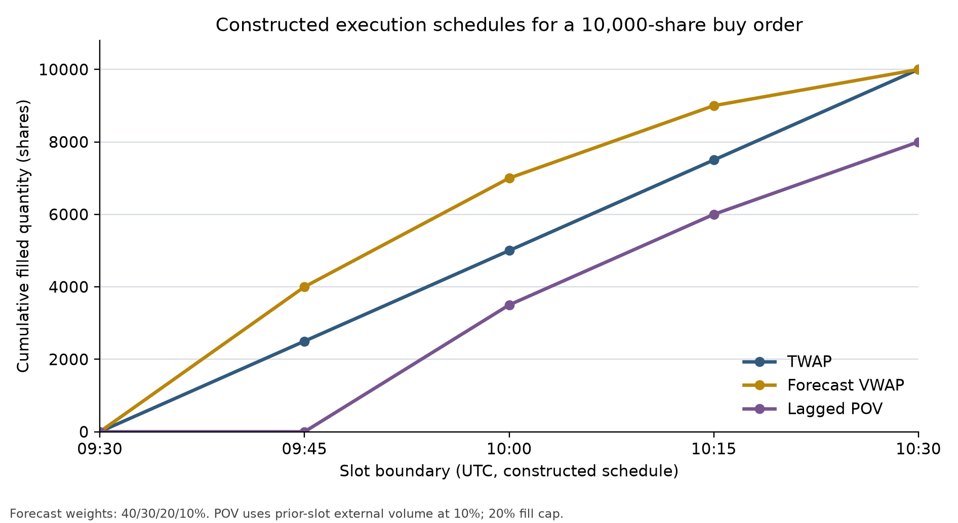
TWAP requests 2,500 shares per slot. Forecast VWAP allocates according to the ex-ante 40/30/20/10% curve. Lagged POV makes no request in the first slot because no volume has yet been observed, then requests 10% of the previous slot's volume, subject to a 20% cap on current external volume. The vertical axis is cumulative shares filled and the horizontal axis is the constructed clock's slot boundaries. POV ends with 2,000 shares remaining.

Figure 2: Discrete Almgren–Chriss Expected Cost and Risk

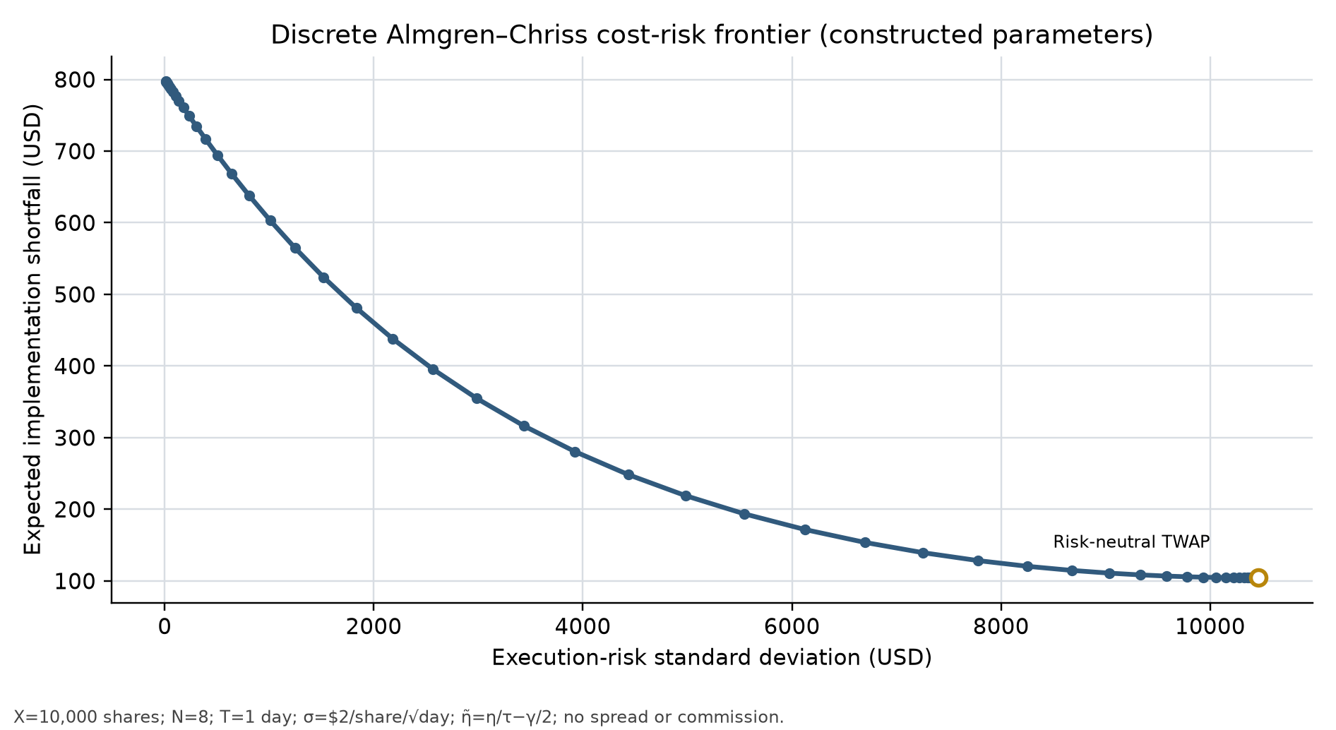
Each point is calculated from the discrete inventory recursion, with a fixed 10,000-share parent order, 8 slots, and a total duration of one day; $\sigma=2$ USD/share/$\sqrt{\text{day}}$, $\eta=10^{-6}$ USD·day/share$^2$, and $\gamma=10^{-7}$ USD/share$^2$, with adjusted temporary-impact coefficient $\tilde\eta=\eta/\Delta t-\gamma/2>0$. Commission and spread are excluded. The risk-neutral endpoint is equal-quantity TWAP; as risk aversion increases, the same constructed model trades higher expected cost for lower execution risk.

11. Evidence Boundary and TCA Study Design

This batch has no real tick-by-tick fills, order-book data, or institutional execution sample. It therefore reports no real-security case or empirical slippage. This section follows the data boundary recorded in qa/a7/ch35_ch36_batch/SOURCE_DATA_GAP.md and offers a study-design example for future work with appropriately authorized data.

11.1 Available Data and Gaps

1. No tick-level or Level 2 feeds. The current course environment contains daily and monthly factor-analysis data, such as Kenneth French industry portfolio returns. It has neither purchased nor mounted full-market historical millisecond trade prints, five- or ten-level order-book snapshots, nor a full-depth message feed such as Nasdaq TotalView-ITCH. The order-book sweeps and slot fills shown in the chapter are constructed for instruction and cannot be used to infer historical tick-level execution slippage for particular US or A-share securities.
2. No borrow or financing series. Historical security-level borrowable lists, borrow-fee rates and hard-to-borrow surcharges, and broker recall records are unavailable. The empirical feasibility of short sales cannot be closed end to end.
3. No broker TCA sample. There are no institutional parent-order execution details for large orders. Values such as square-root impact constants and temporary-impact shares are teaching parameters, not empirical estimates for real markets.

11.2 Example TCA Design with Real Data

With appropriately authorized market and order data, a researcher could preregister the relevant conventions for the question at hand. The steps below are an example analysis workflow, not a universal industry standard:

1. Collect and align data. Record the OMS/EMS parent-order decision timestamp $t_d$, route-send time $t_{\text{send}}$, and exchange fill-confirmation time $t_{\text{fill}}$ at microsecond or nanosecond precision. Align fills to the relevant exchange's consolidated market-data feed.

2. Capture benchmarks.

   • Arrival midpoint: use the national best bid and offer midpoint at the agreed parent-order arrival instant, $P_{\text{arrival}}=(P_{\text{NBBO}}^{\text{bid}}+P_{\text{NBBO}}^{\text{ask}})/2$.
   • Market VWAP: define the trade window and eligible prints according to the research question, market-data source, and benchmark. Inclusion rules for auctions, off-exchange or block prints, corrections, and late reports vary by benchmark and must be documented in advance; do not assume that one set should always be excluded.

3. Factorized impact regression. If appropriately authorized data become available, a future study could regress parent-order slippage on trading characteristics. No estimation is performed in this batch:

   $$\text{Slippage}_i=\alpha+\beta_1\sigma_i\left(\frac{|Q_i|}{\text{ADV}_i}\right)^{0.5}+\beta_2\text{Spread}_i+\epsilon_i$$

   Here $i$ indexes orders, $Q_i$ is signed share quantity (positive for buys and negative for sells), and $\text{ADV}_i>0$ is the security's average daily share volume. Use one day's share volume in the denominator so that $|Q_i|/\text{ADV}_i$ is a fraction of daily volume; do not mix shares with dollar volume. The dependent variable $\text{Slippage}_i$ is a direction-adjusted price deviation in USD/share, for example $\operatorname{sgn}(Q_i)(P_{\text{fill},i}-P_{\text{benchmark},i})$. Both $\sigma_i$, the standard deviation of one-day price changes estimated from a window frozen before the decision, and $\text{Spread}_i$, the full spread, are in USD/share. The intercept $\alpha$ and residual $\epsilon_i$ therefore also have units USD/share, while $\beta_1$ and $\beta_2$ are dimensionless. For a sell order with $Q_i=-1000$ and $\text{ADV}_i=100000$, the original $\sqrt{-0.01}$ is outside the real domain; the corrected value is $\sqrt{0.01}=0.1$. This is a future study design, with no real-data calibration in this batch. Slippage or costs under constructed parameters do not establish real strategy capacity.