Statistical Inference: uncertainty in research conclusions

1. Learning goals

After this chapter, you should formulate a question about an unknown population parameter, choose a sample statistic as an estimator, and interpret the realized estimate. You should derive maximum likelihood estimates (MLEs) of mean and variance under independent normal observations; compute and interpret confidence intervals, p-values and testing errors; distinguish bias, variance, consistency and likelihood; choose resampling for temporal dependence; and perform a small Bayesian update with a clear interpretation of each output.

Record the estimand, observation mechanism and test assumptions beside the result before pressing a test button. Prerequisites are Chapter 6’s expectations, conditional probability, LLN and CLT, and Chapter 4’s differentiation. Chapter 8 extends this inference to regression coefficients.

The statistics script uses core functions in statistics_tools.py; the historical course-root Notebook provides an interactive version. Simulations are labeled constructed samples. Actual industry returns use the French snapshot saved in Chapter 2. These illustrate statistical methods without establishing a tradable strategy.

2. Why a quant needs inference

One backtest reports daily mean return 0.03%, another 0.04%. The second is larger, but if it uses only 20 days during which one news story persists, the difference is not automatically a repeatable advantage. Statistics assesses the strength of conclusions supported by finite, noisy observations, rather than making result tables appear precise.

Quantitative research faces variation in the sample mean, possible changes in the generating mechanism, and searches across many versions with only the best retained. Classical intervals mainly address the first. They do not automatically handle regime changes or record discarded experiments.

An interval can describe instability of a fixed rule’s mean estimate under a specified model. Tradability, costs, information availability and whether the rule was frozen in advance still require financial and experimental design. Chapters 22 and 30–32 develop those parts.

3. Intuition

3.1 One historical path, but a sampling distribution asks about repetition

Imagine randomly weighing a batch of apples from a continually replenished supply. The supply’s mean weight is an unknown population parameter; the batch is a sample. Another batch selected by the same rule yields another mean. Calculating this batch’s mean is arithmetic; studying how means change across batches is inference. The analogy explains repeated sampling only. Markets have time-ordered dependence and regime changes, so trading days are not freely exchangeable apples.

A statistic is a function of the sample, such as its mean. For observed data it is a fixed number; before observation it varies with the random sample and has a sampling distribution. Keep these perspectives separate when reading intervals and tests.

3.2 Standard deviation and standard error describe different variation

Return standard deviation describes single-period volatility. Standard error (SE) describes an estimator’s variability across repeated samples. More independent observations reduce the sample mean’s SE, but downloading ten more years does not reduce the market’s daily volatility.

For example, a daily standard deviation of 2% gives a mean SE of about 0.2% across 100 independent observations. Tomorrow’s return does not thereby fluctuate by only 0.2%. Under the specified model, the estimator formed from the 100-day average has sampling variability of about 0.2%.

3.3 Nonsignificance does not establish absence of an effect

High noise and a small sample can hide a small, real mean effect. Failure to reject zero mean means that this test lacks evidence to reject it. Establishing an economically negligible effect instead requires a prespecified tolerance and equivalence or interval-bound analysis; a large p-value alone cannot establish this.

4. Mathematical foundations

4.1 Samples, parameters and estimands

Specify the estimand too: unconditional mean excess return over a period, or a conditional mean in a market state? An average over surviving securities, or the complete contemporaneous population? Match the reported mean to its target, units, window and sampling unit. An API cannot make these choices for you.

4.2 Sample mean and variance

$\bar X$ is the sample-mean estimator in the units of $X_i$. $S^2$ uses denominator $n-1$ and squared observation units; sample standard deviation $S=\sqrt{S^2}$ shares observation units. Require $n\ge2$. The realized estimates are $\bar x,s^2,s$. Under IID observations and finite second moments, $\mathbb E[\bar X]=\mu$ and $\operatorname{Var}(\bar X)=\sigma^2/n$. Section 6 explains $n-1$.

4.3 From IID to dependence: the full sample-mean variance

Without assuming independence, we still have

Here $\operatorname{Cov}(X_i,X_j)$ is covariance between observations $i,j$. Under weak stationarity, the mean stays constant and lag-$k$ autocovariance is $\gamma_k=\operatorname{Cov}(X_t,X_{t-k})$, giving

$\gamma_0$ is single-period variance. Lag $k$ has $n-k$ observation pairs, occurring in both matrix triangles; this gives factor 2 and $1-k/n$. Zero autocovariance at all nonzero lags suffices to reduce the expression to $\sigma^2/n$. For fixed $n$, nonzero terms may also cancel in the weighted sum. Zero covariance does not generally mean independence.

With absolutely summable autocovariances and suitable weak-dependence assumptions, define long-run variance $\Omega=\gamma_0+2\sum_{k=1}^\infty\gamma_k$; large-sample mean variance is approximately $\Omega/n$. Chapter 8 introduces heteroskedasticity and autocorrelation consistent (HAC) standard errors. Writing SE as $s/\sqrt n$ already invokes an important assumption.

5. Definitions

5.1 Bias, variance and mean squared error

$\hat\theta=T(X_1,\ldots,X_n)$ is an estimator. Subscript $\theta$ denotes expectation under a model with parameter $\theta$; MSE means mean squared error. These definitions concern scalar parameters; matrix parameters need a specified loss function. Zero bias means unbiasedness.

Consistency means that an estimator approaches the true parameter in probability as sample size tends to infinity: for any $\varepsilon>0$,

Unbiasedness concerns expectation at each finite sample size; consistency concerns the limit of an estimator sequence. Neither replaces the other. When adding market observations, ask whether the mechanism needed for that limit still applies.

Bias measures average deviation across repeated samples; variance measures spread across samples; consistency asks whether errors vanish in probability with increasing sample size; MSE combines variance and squared bias in one loss scale. They describe finite-sample center, dispersion, limiting behavior and squared loss respectively.

5.2 Likelihood and maximum likelihood

For IID continuous observations, the likelihood function is

$f_\theta$ is model density, $x$ fixed observed data, and $\Theta$ the permitted parameter space. For discrete data use PMFs instead. Likelihood fixes the data and varies the parameter. A continuous variable has zero probability at an exact point, so we compare densities, not the probability of this exact decimal sequence. Likelihood is not posterior parameter probability.

Dependence requires a joint or conditional distribution, for example $f_\theta(x_1)\prod_{t=2}^n f_\theta(x_t\mid x_{1:t-1})$. Multiplying marginal densities instead actively substitutes a different model.

Bias, variance and consistency characterize estimators’ average deviations, repeated-sample spread and large-sample convergence. Likelihood compares parameter values’ relative fit for fixed data. Its value is neither a parameter probability nor a description of sampling variability.

5.3 Confidence intervals, tests and errors

An interval procedure $[L(X),U(X)]$ has confidence level $1-\alpha_{\mathrm{sig}}$ if its coverage satisfies

or reaches at least the target level where appropriate. $L,U$ are random endpoints, $\theta$ a fixed parameter, and $\alpha_{\mathrm{sig}}$ the significance level, distinct from asset-pricing alpha. Approximate intervals can have coverage different from nominal; assess that approximation.

A hypothesis test specifies null $H_0$ and alternative $H_1$, then its statistic and rejection region. Type I error rejects a true $H_0$. Type II error fails to reject under a specified true alternative. Power is the probability of rejecting $H_0$ under that alternative, or one minus Type II error probability. It depends on effect size, noise, sample size and the decision rule; it is not one fixed property of a test.

For this chapter’s two-sided t test, a p-value is the null-model probability of a statistic at least as extreme as observed. It is neither the probability that $H_0$ is true nor a strategy’s failure probability.

5.4 Bootstrap and Bayesian inference

Bootstrap uses observations to approximate an unknown generating distribution and repeatedly recalculates the statistic to approximate sampling variability. Resampling must preserve the structures relevant to the question.

Bayesian inference represents parameter uncertainty with a probability distribution. Prior, likelihood and posterior satisfy

$\pi(\theta)$ is prior density, the denominator is marginal data density, and $u$ the integration variable. Use sums for discrete parameters. Posterior probability statements condition on the model and prior. A credible interval contains a specified posterior mass and differs in meaning from a frequentist confidence interval.

Frequentist inference fixes the parameter and varies data across repeated samples; confidence describes the procedure’s long-run coverage. Bayesian inference assigns posterior parameter probabilities given the model, prior and observed data. Posterior mass and coverage describe different uncertainty objects.

6. Derivations

6.1 Why sample variance divides by $n-1$

Start with the algebraic identity:

$\mu$ is the common population mean. Expanding $X_i-\bar X=(X_i-\mu)-(\bar X-\mu)$ gives cross-term sum $-2n(\bar X-\mu)^2$; adding $n(\bar X-\mu)^2$ yields the identity.

Under IID observations with finite variance, the first right-hand term has expectation $n\sigma^2$ and the second $n\operatorname{Var}(\bar X)=\sigma^2$. The squared-deviation sum therefore has expectation $(n-1)\sigma^2$, so dividing by $n-1$ gives an unbiased variance estimator. Estimating the common center makes residuals sum to zero, leaving $n-1$ free directions.

For correlated observations, $\operatorname{Var}(\bar X)$ generally differs from $\sigma^2/n$, so this unbiasedness derivation cannot be reused unchanged. ddof=1 states a computation convention; it does not prove IID data.

6.2 Gaussian mean and variance MLEs

Assume $X_i\overset{\mathrm{IID}}\sim N(\mu,v)$ with $v=\sigma^2>0$. The log-likelihood is

$\ell$ is the natural log of likelihood. A strictly increasing logarithm preserves the maximizer. Differentiate with respect to $\mu$:

Substitute $\bar x$ and differentiate with respect to $v$:

With a positive squared-deviation sum, profile log-likelihood tends to negative infinity as $v\to0$ and $v\to\infty$; its stationary point is the maximum. If all $x_i$ are identical, the sum is zero. Setting $\mu$ to that common value makes likelihood grow without bound as $v\downarrow0$. There is no finite MLE in the regular Gaussian model with $v>0$. A descriptive zero variance is not a valid regular Gaussian MLE; the core function raises an explicit error.

Note that

The variance MLE is downward biased but remains consistent under IID observations, finite second moments and the relevant LLN. MLE need not be unbiased; finite- and large-sample properties differ.

6.3 Bias–variance decomposition of MSE

Write the estimation error as

Square and take expectation. The cross term contains $\mathbb E[\hat\theta-\mathbb E\hat\theta]=0$, hence

This explains the value of shrinkage. Pulling extreme estimates toward a common center introduces bias, but a sufficiently large variance reduction can lower total error. Chapter 8 uses this in regularized regression and Chapter 21 in covariance shrinkage.

6.4 The t interval for an IID normal mean

$t_{n-1}$ is Student’s t with $n-1$ degrees of freedom. Estimating unknown volatility adds uncertainty and gives small-sample t heavier tails than normal. Independence of the normal sample mean and squared deviations follows from orthogonal Gaussian components. This chapter states that distribution fact without fully proving the chi-squared density.

Choose critical value $q=t_{n-1,1-\alpha_{\mathrm{sig}}/2}$ so that $\Pr(-q\le T\le q)=1-\alpha_{\mathrm{sig}}$. Because $S/\sqrt n>0$, rearrangement gives

$q$ is dimensionless, $S/\sqrt n$ the mean’s SE, and endpoints share return units. This is an exact IID Gaussian interval. Nonnormal independent samples require separate asymptotic assumptions and finite-sample checks. A large dependent sample alone cannot recover the exact result.

For testing $H_0:\mu=\mu_0$, use $t_{\mathrm{obs}}=(\bar x-\mu_0)/(s/\sqrt n)$ and two-sided p-value $2\Pr(t_{n-1}\ge |t_{\mathrm{obs}}|)$. With the same assumptions and two-sided level, $\mu_0$ outside the corresponding interval is equivalent to rejecting $H_0$. Different SEs or one-/two-sided rules break that direct correspondence.

6.5 Constructing a percentile bootstrap interval

After observing $x_1,\ldots,x_n$, the empirical distribution places mass $1/n$ at each observation. Each IID bootstrap replication samples $n$ entries with replacement and computes $\bar x^{*(b)}$, for $b=1,\ldots,B$. A star marks resampling and $B$ is replication count. The percentile interval uses quantiles $\alpha_{\mathrm{sig}}/2$ and $1-\alpha_{\mathrm{sig}}/2$ of those means.

The empirical distribution approximates the unknown population, and repeated empirical samples approximate the estimator’s sampling variation. Finite-sample bias, skewness, heavy tails, nonsmooth statistics and boundary parameters can impair coverage. Increasing $B$ mainly reduces Monte Carlo error in resampling calculations; it creates no new market observations.

Independent day-by-day resampling destroys neighboring relationships in a financial sequence. Mean inference then misses temporal covariance’s contribution to SE. Justify an IID approximation before applying independent bootstrap to financial data.

For time series, sample blocks of neighboring observations instead. Here a circular block bootstrap uses fixed length $L$: choose random starts, preserve within-block order, wrap at the sample’s end, concatenate and truncate to $n$ observations. It retains short-term within-block dependence but cuts relationships at joins; the circular boundary is itself an approximation. Short blocks can omit dependence, while long blocks offer fewer effective rearrangements. Wider intervals alone do not establish correctness.

Asymptotic validity of block methods requires stationarity, relevant moments and sufficiently decaying dependence, among other assumptions. Common results also require $L\to\infty$ and $L/n\to0$. These two rate conditions are not complete theorem assumptions and do not guarantee a fixed $L=12,n=180$ setting. Künsch’s original study concerns block resampling of general stationary observations (Section 20); this chapter uses a circular fixed-block variant to illustrate structure.

6.6 Beta–Binomial updating

Assume $Y_i\mid p\overset{\mathrm{IID}}\sim\operatorname{Bernoulli}(p)$ and observe $s$ successes and $f$ failures. Prior $p\sim\operatorname{Beta}(a,b)$ with $a,b>0$ has density kernel $p^{a-1}(1-p)^{b-1}$; likelihood kernel is $p^s(1-p)^f$. Multiplication gives

$p$ is success probability, $a,b$ dimensionless prior shape parameters, and $s,f$ counts. A posterior remaining in the prior distribution family is conjugate. Its mean is

where $n=s+f>0$. This is a weighted average of prior mean and sample success rate. It does not mean the prior contains (a+b) real observed trades; the weights have an algebraic interpretation. Explain the prior’s economic basis and assess sensitivity.

6.7 Power and sample size: detecting a small effect

To examine power, temporarily assume IID Gaussian observations with known single-period standard deviation $\sigma$. Prespecify one-sided hypotheses $H_0:\mu=0$ and $H_1:\mu>0$. A directional hypothesis must precede the research; a positive observed mean does not justify switching from two-sided to one-sided.

Let $c=z_{1-\alpha_{\mathrm{sig}}}$ and reject when $\sqrt n\bar X/\sigma>c$. Under specified alternative $\mu=\delta>0$, this statistic follows $N(\sqrt n\delta/\sigma,1)$, hence

$\Phi$ is the standard-normal CDF, $\delta$ the prespecified effect in single-period return units, and $n$ independent-observation count. With fixed significance, a larger effect, lower noise or more independent observations increases power. Type II error is one minus power under that alternative, not the probability of an ineffective strategy after nonrejection.

For target power $1-\beta_{\mathrm{II}}$, rearrangement gives the sample-size design bound, rounded up to a minimum integer:

$\beta_{\mathrm{II}}$ is the Type II error target, not market beta. With single-period standard deviation 2%, target mean 0.1%, one-sided level 5% and power 80%, round upward to 2474 independent observations. As trading days, these span years; adding data may also introduce mechanism changes. This idealized sample size is not a market-research guarantee.

import numpy as np
from scipy import stats

sigma, delta, significance, target_power = 0.02, 0.001, 0.05, 0.80
critical = stats.norm.ppf(1.0 - significance)
required = int(np.ceil((sigma / delta * (critical + stats.norm.ppf(target_power)))**2))
for n in (100, 1000, required):
    power = stats.norm.sf(critical - np.sqrt(n) * delta / sigma)
    print("known-sigma IID Gaussian, one-sided", n, "power", power)
assert stats.norm.sf(critical - np.sqrt(required) * delta / sigma) >= target_power

This design illustration does not use unknown-standard-deviation t power, temporal dependence or multiple testing. Recalculate or simulate under the research model; 2474 is not a universal strategy acceptance threshold.

7. Financial interpretation

7.1 Measure payoffs, not win rate alone

Suppose each win earns 1 unit, each loss loses 2 units, every trade costs 0.1 unit, and success probability is $p$. Expected net payoff per trade is

$G$ is net payoff per trade, so a positive expectation requires $p>0.7$. Even a high posterior probability that $p$ exceeds 0.5 cannot establish positive expected strategy returns. This example fixes payoff magnitudes; actual amounts, holding times and tail risk need separate modeling.

7.2 Effect size, statistical significance and economic value

Statistical significance assesses incompatibility with the tested hypothesis. Economic value assesses whether an effect warrants costs and risk given capacity.

A daily gross mean of 0.02% with costs 0.03% has a negative net mean even if a large sample estimates the gross mean precisely. A positive mean with a wide interval may instead leave economic value uncertain. Report effect size, interval, cost convention and risk alongside one another; a p-value is not a sole strategy-ranking score.

A mean significantly different from zero also does not remove market beta. Long exposure in a rising market can have a positive mean without independent alpha. Chapters 14–15 specify asset-pricing and factor-regression benchmarks.

7.3 Effective sample size: intuition and scope

For stationary first-order autoregression (AR(1)) $X_t-\mu=\phi(X_{t-1}-\mu)+\varepsilon_t$, assume $|\phi|<1$ and independent zero-mean innovations with finite variance. Then $\gamma_k=\gamma_0\phi^{|k|}$. Substituting the geometric series into long-run variance gives

$n_{\mathrm{eff}}$ is effective sample size that approximately matches an independent mean variance, not actual independent-trade count. It is a large-sample stationary AR(1) approximation for mean estimation, not a replacement for every model’s degrees of freedom. At $n=180,\phi=0.7$ the approximation is 31.76: 180 rows need not provide 180 independent information units. Negative correlation can reduce mean variance; $n_{\mathrm{eff}}>n$ is not a mathematical error.

8. Numerical Example

8.1 Four returns calculated by hand

8.2 Recorded fixed-seed outputs

The full script uses seed 20261007 and independent child streams for experiments. Forty constructed IID Gaussian observations have model mean 0.002 and standard deviation 0.02. The recorded realization has sample mean about −0.001500, variance MLE about 0.00045812, unbiased variance about 0.00046987, 95% interval $[-0.008432,0.005432]$ and zero-mean p-value about 0.664051. The difference between true mean and realized estimate is the point of this experiment.

Across 3000 correct-model experiments, 95% t coverage at sample sizes 10, 30 and 100 was about 95.3333%, 94.9333% and 95.5%. A finite simulation need not yield exactly 95%. At true coverage 0.95, the SE of 3000 coverage indicators is approximately $\sqrt{0.95\times0.05/3000}=0.003979$, or 0.398 percentage points. This is Monte Carlo error in simulated coverage, not a market-return SE.

The stationary constructed AR(1) sample contains 240 observations; the first 180 enter estimation, while the final 60 stay out of resampling. With $\phi=0.7$ and innovation standard deviation 0.01, 4000 resamples gave an IID percentile interval about $[-0.002327,0.001643]$ and a circular length-12 block interval about $[-0.003428,0.002961]$. Blocks were wider for this particular sample; greater width is neither a universal theorem nor proof of coverage. Repeated generation and block-length sensitivity require separate checks.

Finally, prior Beta(2,2) and 6 wins/4 losses give posterior Beta(8,6), with success-probability mean $8/14=4/7\approx0.571429$. Using Section 7’s payoff structure gives posterior expected net payoff $3\times4/7-2.1\approx-0.385714$ units/trade.

9. Python Implementation

Default entry point in the accepted reader package

From the accepted I3 reader package root, create the isolated environment described in its README, then run:

.venv/bin/python run_notebook.py notebooks/ch07_statistics.ipynb

This notebook calls the packaged shared implementation, reads no omitted French data and downloads nothing. Each execution writes a unique UUID subdirectory under runs and prints its location. Old production tests and historical course-root commands below belong to the original project; the default reader route is this package-root notebook with its assertions. Optional historical French inputs follow the reader’s data contract; this batch did not rerun them.

Historical course-root route

Run the following self-contained blocks from the course root using the course environment. Each supplies its imports and data. Core functions require one-dimensional finite numeric observations and do not silently discard NaNs, which could change the observation window. Before deleting missing values, investigate dates and causes as in Chapter 3 and record them.

9.1 Check estimates, intervals and tests together

import numpy as np
from scipy import stats
from quant_course.statistics_tools import (
    normal_mle_estimates, mean_t_confidence_interval, one_sample_t_test,
)

sample = np.array([-0.01, 0.01, 0.02, 0.02], dtype=float)
estimates = normal_mle_estimates(sample)
interval = mean_t_confidence_interval(sample, confidence_level=0.95)
test = one_sample_t_test(sample, null_mean=0.0)
assert np.isclose(estimates.mean, 0.01)
assert np.isclose(estimates.variance_mle, 0.00015)
assert np.isclose(estimates.variance_unbiased, 0.0002)
reference = stats.ttest_1samp(sample, popmean=0.0)
assert np.isclose(test.p_value, reference.pvalue)
assert (interval.lower <= 0.0 <= interval.upper) == (test.p_value >= 0.05)
print(estimates)
print(interval)
print(test)

These estimate a single-period mean, not annualized return, with no signal or order time. The interval object’s standard_error is the mean’s SE, not daily-return volatility. SciPy checks computation; you remain responsible for model assumptions.

9.2 Explicit failure for constant or missing samples

import numpy as np
from quant_course.statistics_tools import normal_mle_estimates

constant = np.array([0.01, 0.01, 0.01])
assert constant.var(ddof=0) == 0.0
for invalid in (constant, np.array([0.01, np.nan, 0.02])):
    try:
        normal_mle_estimates(invalid)
    except ValueError as error:
        print(type(error).__name__, str(error))
    else:
        raise AssertionError("invalid input must not produce a regular Gaussian MLE")

A constant sample can have descriptive variance zero, yet no regular Gaussian MLE exists in parameter space $v>0$. These statements are consistent. Replacing the error with zero-filled continuation would hide the failure.

9.3 Resampling that preserves dependence

import numpy as np
from quant_course.statistics_tools import (
    simulate_stationary_ar1, bootstrap_mean_draws,
    moving_block_bootstrap_mean_draws, bootstrap_mean_confidence_interval,
)

streams = [np.random.default_rng(s) for s in np.random.SeedSequence(20261017).spawn(3)]
observations = simulate_stationary_ar1(
    n=240, phi=0.7, innovation_std=0.01, rng=streams[0],
)
train = observations[:180]
holdout = observations[180:]
assert len(holdout) == 60
point_estimate = float(train.mean())
iid = bootstrap_mean_draws(train, n_resamples=2000, rng=streams[1])
blocks = moving_block_bootstrap_mean_draws(
    train, block_length=12, n_resamples=2000, rng=streams[2],
)
for name, draws in (("IID", iid), ("circular fixed blocks", blocks)):
    interval = bootstrap_mean_confidence_interval(draws)
    print(name, "original mean", point_estimate, "interval", interval)

Each method in this block uses 2000 resamples; Section 8’s 4000 belong to the full script. The seeds also differ, so do not tune this output to match Section 8. The percentile-interval function returns estimate as the average of the finite set of resampled means, which can differ slightly from the original mean. Code therefore stores the original mean separately as point_estimate. The standard deviation of Section 8’s 4000 resampled means estimates the original mean’s sampling SE. Do not divide it again by $\sqrt{4000}$ to obtain that SE: doing so mistakes computation count for market sample size.

9.4 Bayesian updating and posterior intervals

import numpy as np
from scipy import stats
from quant_course.statistics_tools import beta_binomial_posterior

posterior = beta_binomial_posterior(
    successes=6, failures=4, prior_alpha=2.0, prior_beta=2.0,
)
a, b = posterior.posterior_alpha, posterior.posterior_beta
credible_interval = stats.beta.ppf([0.025, 0.975], a=a, b=b)
probability_above_half = stats.beta.sf(0.5, a=a, b=b)
expected_net_payoff = 3.0 * posterior.posterior_mean - 2.1
assert np.isclose(posterior.posterior_mean, 4.0 / 7.0)
assert expected_net_payoff < 0.0
print("posterior", posterior)
print("95% equal-tail credible interval", credible_interval)
print("posterior P(p > 0.5)", probability_above_half)
print("posterior expected net payoff, units per trade", expected_net_payoff)

This is a 95% equal-tail credible interval, leaving 2.5% posterior mass at each end. It is neither a frequentist coverage-guaranteed interval nor a highest-posterior-density interval. .sf(0.5) gives posterior probability under the specified Beta–Binomial model and prior, with a meaning different from a t-test p-value.

10. Visualization

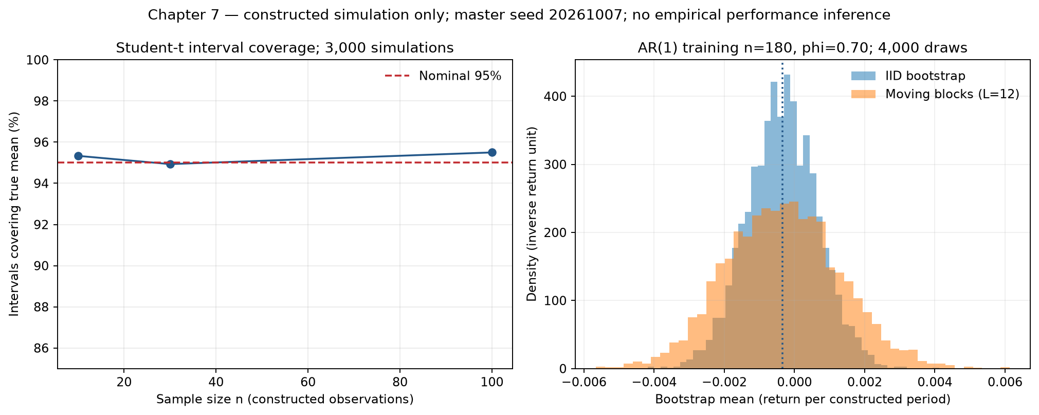
The left panel’s horizontal axis is sample size per simulation and its vertical axis the proportion of 3000 independent experiments covering the true mean. The dashed line is nominal 95%. Observe finite-simulation fluctuations around that level; one point slightly above it does not establish superiority. This checks the specified IID Gaussian experiment, not normality or independence of real returns.

The right panel shows resampled means from the first 180 AR(1) observations, in decimal-return units. Its vertical axis is density, in reciprocal-return units; each histogram has area approximately 1. Blocks are more dispersed in this sample because they retain some positive serial dependence. They include no future 60 observations and use no holdout outcomes to tune block length.

Distinguish raw-return distribution, the mean’s sampling distribution, and the finite-sample bootstrap approximation. The figure shows the third, not a predictive interval for the next return.

11. Real Market Example

Use the saved French 10-industry monthly-return snapshot, prespecify January 2010–December 2019 as the descriptive window, and select Non-durables (NoDur). Fix the range and verify consecutive months before computing mean and an IID reference interval. “Reference” matters: executing code does not establish independent normal observations in this real-market sequence.

from pathlib import Path
import numpy as np
import pandas as pd
from quant_course.statistics_tools import mean_t_confidence_interval

raw = pd.read_csv(
    Path("data/processed/french_10_industries_monthly.csv"), dtype={"month": "string"},
)
monthly = raw.set_axis(pd.PeriodIndex(raw.pop("month"), freq="M"), axis="index")
series = monthly.loc["2010-01":"2019-12", "NoDur"]
expected = pd.period_range("2010-01", "2019-12", freq="M")
assert series.index.equals(expected)
assert np.isfinite(series.to_numpy()).all()
reference = mean_t_confidence_interval(series.to_numpy())
print("published monthly industry snapshot; not a PIT tradable security")
print("n", len(series), "sample mean", float(series.mean()))
print("IID Gaussian reference interval; assumptions unverified", reference)
print("lag-one sample correlation, diagnostic only", float(series.autocorr(lag=1)))

No automatic .dropna() occurs; missing data fail the checks. Monthly labels identify published portfolios’ return months, not proof that data were public at that month-end. The recorded snapshot calculation gave monthly mean about 1.009917%, an IID-reference 95% interval about [0.428369%,1.591465%], and lag-one sample correlation about −0.188911; see the snippet record. These are window-specific calculations, not independence evidence. Near-zero sample lag correlation does not prove independence, and volatility clustering can retain dependence elsewhere. Chapters 16–18 examine serial and volatility structure; Chapter 8 introduces HAC inference.

Industry-portfolio return is not active-strategy excess return, and these data do not subtract the tutorial’s actual trading costs. Record the outputs as descriptive statistics and reference-model calculations for that window, rather than claiming future monthly means will lie between the endpoints. The downloaded version can revise history; point-in-time (PIT) conditions remain unmet. Cache notes record provenance and hashes.

12. Common Mistakes

12.1 Treating a p-value as null-hypothesis probability

An incorrect claim is: “p=0.03 means only a 3% chance that zero returns are true.” Testing assumes the null and calculates a statistic’s tail probability; it supplies no prior or posterior for the hypotheses. Report model, statistic, two-sided rule, p-value, effect estimate and interval.

12.2 Reading a mean interval as tomorrow’s return range

A mean confidence interval estimates a parameter. A prediction interval also includes a new observation’s randomness. More precise mean estimates can coexist with a wide distribution of tomorrow’s return. Confusing the two understates single-period loss risk.

12.3 Treating more bootstrap replications as more data

12.4 Dropping NaNs without reporting selection

Missing crisis-period prices can raise a mean if their dates are deleted. Missingness itself may relate to returns. In financial data, dropna() selects a sample; report removed dates, proportions and causes rather than treating it as an economically neutral cleaning step.

12.5 Reporting one significant result from 100 attempts

Assume 100 independent tests, all null hypotheses true, and each Type I error exactly 5%. Probability of at least one false rejection is

Here 100 counts attempts, not observations. Independence is a demonstration assumption; correlated strategy tests cannot directly use this equality. Even without knowing the total error rate, selecting the smallest p-value and interpreting it as one isolated test changes the research procedure.

import numpy as np
from scipy import stats

rng = np.random.default_rng(20261027)
null_samples = rng.normal(0.0, 1.0, size=(100, 60))
p_values = stats.ttest_1samp(null_samples, popmean=0.0, axis=1).pvalue
raw_rejections = int((p_values < 0.05).sum())
bonferroni_rejections = int((p_values < 0.05 / len(p_values)).sum())
assert bonferroni_rejections <= raw_rejections
print("100 independent null experiments; simulation only")
print("unadjusted rejections", raw_rejections)
print("Bonferroni rejections", bonferroni_rejections)
print("all-null independent probability of at least one raw rejection", 1 - 0.95**100)

Bonferroni correction divides the family’s target level by test count and uses the union bound to control at least one Type I error. It does not require independence, but may be conservative. This example defines the test family in advance. Unrecorded features, windows and universes mean the final 100 retained tests may not be the full attempt count. Chapter 32 covers multiple testing, selection-adjusted performance and overfitting probability.

13. Quant Research Application

13.1 Write an inference contract before experimenting

For a fixed signal’s mean net return, specify population, universe formation, dates, return interval, data availability, execution time, costs, test target, one-/two-sided rule, dependence treatment and parameter-search scope. Freeze splits and record every attempt. These details let a reader identify the question a result addresses.

These pure inference examples create no holdings, so signal_time and trade_time are inapplicable. Strategy returns instead must come from previously specified executable holdings and a cost model. The statistics module does not detect upstream signal leakage; Chapters 29–31 address backtesting and validation.

13.2 A rejection region is not an investment decision

Investment decisions need estimated net effects, uncertainty, tail/liquidity risks and resource constraints. Nonrejection can lead to further data collection; rejection can still lead to stopping because of capacity, exposures or failed replication. Separate statistical outputs from research-team decisions.

A mean-only model does not establish safe extreme drawdowns. Tail observations are scarce, and resampling can repeatedly replay the same few extremes. Chapter 33 develops VaR, Expected Shortfall and stress scenarios.

13.3 Study robustness rather than search for the best p-value

Prespecify reasonable block lengths, economic subperiods and cost scenarios, and report all of them. Trying settings until an interval excludes zero and reporting only that setting creates another parameter search. Sensitivity analysis should explain which assumptions matter, not select the most favorable conclusion.

14. Chapter Summary

Parameters are study targets, statistics are sample functions, and estimates are realized numbers. Unbiasedness, consistency and low MSE address different questions. Variance MLE divides by $n$; unbiased sample variance divides by $n-1$, with its unbiasedness relying on IID assumptions.

Confidence intervals describe procedural coverage and p-values null-model extremeness. Exact t inference requires independent normal observations. Dependence changes sample-mean variance; suitable block resampling or HAC can address some dependence under assumptions and diagnostics. A Bayesian posterior expresses conditional uncertainty differently; posterior win rates still cannot replace net-payoff analysis.

Completion means being able to state an output’s object, units, window, assumptions and interpretation, beyond obtaining a test-function result.

15. Exercises

7-E01 (identify objects). A researcher says an industry’s 120 monthly returns over 2010–2019 average 1%. Identify observations, estimator, estimate and possible estimand. Does the sample mean automatically equal a future population mean?

7-E02 (hand calculation). For $(-0.01,0.01,0.02,0.02)$, calculate mean, squared-deviation sum, variance MLE, unbiased variance, mean SE and 95% t interval. Why do the two variances differ?

7-E03 (MSE). Two scalar estimators have bias/variance $(0,0.04)$ and $(0.10,0.01)$. Which do you choose under squared loss? Does this make unbiased estimators universally undesirable?

7-E04 (interval language). Distinguish “95% of parameters lie in this computed interval” from “the procedure covers a fixed parameter in about 95% of repeated samples.” Also distinguish mean intervals and prediction intervals for new returns.

7-E05 (effective sample size). For stationary AR(1) with $n=180,\phi=0.7$, calculate large-sample mean effective sample size and SE relative to IID. Repeat for $\phi=-0.3$ and state assumptions.

7-E06 (multiple tests). For 20 independent true-null tests each at 5%, find the probability of at least one false rejection and the per-test Bonferroni level for family level 5%. Which conclusion does not require independence?

7-E07 (prior and payoff). Update Beta(2,2) with 6 wins and 4 losses. Give posterior distribution and mean. With win payoff 1, loss 2 and cost 0.1, find posterior expected net payoff and the success probability required for positive expectation.

7-N01 (identify objects). Study a fixed rule’s mean daily return over a specified window. Identify unknown population parameter, random variable, realized observation, estimator, estimate and sampling unit. Explain repeated sampling here and the information a sampling mechanism must preserve for neighboring-dependent returns.

7-N02 (one calculation). A prespecified right-sided test observes $z=1.50$ with $\Phi(1.50)=0.9332$. Compute the one-sided p-value and decision at $\alpha=0.05$. What does this say about the probability of the null?

7-N03 (complete calculation). Each unit is one independent measurement in common output units. Four IID normal observations are $(1,1,3,3)$ and known population standard deviation $\sigma=2$. Test $H_0:\mu=0$ against $H_1:\mu>0$ at $\alpha=0.05$ with exact critical value $z_{0.95}\approx1.645$. Given approximate CDF values $\Phi(1.645)\approx0.9500$, $\Phi(2)\approx0.9772$ and $\Phi(1)\approx0.8413$, find mean, SE, statistic, p-value, one-sided 95% lower bound and Type I error. At specified approximate alternative $\mu_1=2.645$, find Type II error and power.

7-N04 (code diagnosis). A prespecified right-sided normal test uses p = 2 * (1 - Phi(z)). When does this equal a two-sided p-value, and when does it fail? Correct it to a right-tail formula and compute the result using $z=1.50$ and $\Phi(1.50)=0.9332$. What happens to the two formulas for negative $z$?

7-N05 (research judgment). A researcher selects the best of 40 strategy versions and reports IID right-sided $p=0.03$, gross daily mean 0.02% and daily costs 0.03%. Returns have positive serial correlation. Which statements hold, and which claims lack support? Give at least three reporting or checking requirements.

16. Programming Exercises

7-P01 (cross-check computation). Independently generate 80 normal observations with seed 20261037, mean 0.001 and standard deviation 0.02. Calculate a 95% t interval and zero-mean test with the core functions, then cross-check SciPy and assert their two-sided correspondence. Do not make the assertion depend on whether this realization is significant.

7-P02 (block-length sensitivity). With seed 20261047, generate 300 stationary AR(1) observations. Use the first 240 as training and leave 60 unused. For lengths 4, 12 and 24, use independent streams and 2000 circular block resamples, recording intervals and widths. Do not choose block length by zero-mean rejection.

7-P03 (prior sensitivity). Keep 6 wins/4 losses fixed and use Beta(1,1), Beta(2,2) and Beta(10,10). Compute posterior means, 95% equal-tail credible intervals and expected net payoffs. Explain stronger-prior shrinkage toward 0.5 and why interval changes are not additional trading evidence.

17. Challenge Problems

7-C01 (finite-sample dependence). Derive stationary AR(1) mean variance at finite $n$ from the double sum. At $n=180,\phi=0.7$, compare finite-sample SE inflation with its long-run approximation and explain omitted boundary weights. Do not treat effective sample size as universal model degrees of freedom.

7-C02 (design coverage experiments). Compare IID t, IID bootstrap and circular length-12 bootstrap coverage under IID Gaussian and stationary AR(1) generation. Specify true mean, sample size, outer replications, bootstrap repetitions, random streams, coverage/width metrics, simulation error and limits for market conclusions. Do not require a preselected winner.

18. Solutions / Solution Hints

7-E01

Observations are the 120 specified monthly industry-portfolio returns. Estimator is $\bar X=(1/120)\sum_{t=1}^{120}X_t$ and estimate 0.01. The estimand could be monthly industry mean under a stationary generating model, or simply a fixed-window descriptive average; choose and state which. A changed future distribution prevents automatic estimation of its mean. Industry portfolios, security populations and tradable strategies are different objects.

7-E02

Sum 0.04 divided by 4 gives 0.01. Deviations −0.02, 0, 0.01 and 0.01 give squared sum 0.0006. Dividing by 4 gives MLE variance 0.00015, and by 3 sample variance 0.0002. Standard deviation is $\sqrt{0.0002}\approx0.0141421$; divide by 2 for mean SE about 0.0070711. Multiplying by the 3-degree critical value 3.182446 gives half-width about 0.0225033 and interval [−0.0125033,0.0325033]. MLE maximizes model density; division by $n-1$ targets unbiasedness under IID finite second moments. Different purposes give different denominators.

7-E03

The first MSE is 0.04 and the second $0.01+0.10^2=0.02$, so choose the second here. This compares squared loss at specified parameters; other losses, bias directions or parameter spaces can change the choice. It refutes universal superiority of unbiasedness, not all usefulness of unbiased estimation.

7-E04

Frequentist parameters are fixed and data/endpoints random; the interval-generating procedure repeats. After observation the interval is fixed, and assigning 95% probability to a fixed parameter needs an additional parameter-probability model. Bayesian posteriors permit parameter probabilities conditional on model and prior. Mean intervals address estimation error; prediction intervals add new-observation randomness and are usually wider. Mechanism changes can invalidate either despite their mathematical form.

7-E05

$n_{\mathrm{eff}}\approx180\times0.3/1.7=31.7647$, with SE inflation about $\sqrt{(1+0.7)/(1-0.7)}\approx2.38048$. For $\phi=-0.3$, effective sample size is approximately $180\times1.3/0.7\approx334.286$ and SE ratio $\sqrt{0.7/1.3}\approx0.733799$. Negative correlation reduces mean variability; it does not create independent observations. These results require stationary AR(1), finite second moments and a large-sample approximation, not an unconditional substitution for t degrees of freedom.

7-E06

Under independence, probability of at least one error is $1-0.95^{20}\approx0.641514$. The Bonferroni per-test level is $0.05/20=0.0025$. The first equality requires independence. The union bound applies to arbitrary events, so Bonferroni’s family-error bound does not; however, individual tests must be valid and the family and attempts correctly recorded.

7-E07

Posterior is Beta(8,6), with mean $8/14=4/7$. Expected net payoff is $3\times4/7-2.1=-0.385714$ units/trade. Under fixed payoffs and costs, break-even success probability is 0.7 and strictly positive expectation requires $p>0.7$. A win rate above one half does not offset larger losses and costs.

7-P01

The reference implementation follows. Changing seeds may change significance, but computational correspondence should remain.

import numpy as np
from scipy import stats
from quant_course.statistics_tools import mean_t_confidence_interval, one_sample_t_test

sample = np.random.default_rng(20261037).normal(0.001, 0.02, size=80)
interval = mean_t_confidence_interval(sample)
test = one_sample_t_test(sample)
reference = stats.ttest_1samp(sample, popmean=0.0)
assert np.isclose(test.t_statistic, reference.statistic)
assert np.isclose(test.p_value, reference.pvalue)
assert (interval.lower <= 0.0 <= interval.upper) == (test.p_value >= 0.05)
print(interval, test)

Scoring: self-contained data and code; a t statistic using ddof=1; daily-return units; no interpretation of p-values as strategy-validity probabilities.

7-P02

import numpy as np
from quant_course.statistics_tools import (
    simulate_stationary_ar1, moving_block_bootstrap_mean_draws,
    bootstrap_mean_confidence_interval,
)

streams = [np.random.default_rng(s) for s in np.random.SeedSequence(20261047).spawn(4)]
series = 0.001 + simulate_stationary_ar1(
    n=300, phi=0.7, innovation_std=0.01, rng=streams[0],
)
train, holdout = series[:240], series[240:]
assert len(holdout) == 60
for length, rng in zip((4, 12, 24), streams[1:]):
    draws = moving_block_bootstrap_mean_draws(
        train, block_length=length, n_resamples=2000, rng=rng,
    )
    interval = bootstrap_mean_confidence_interval(draws)
    print(length, interval.lower, interval.upper, "width", interval.upper - interval.lower)

Widths need not be monotone. Finite-sample and resampling randomness can change their order. Report all three prespecified settings, explain dependence missed by short blocks and fewer rearrangements with long blocks, and use neither holdout mean nor zero exclusion to select length.

7-P03

from scipy import stats
from quant_course.statistics_tools import beta_binomial_posterior

for prior in (1.0, 2.0, 10.0):
    posterior = beta_binomial_posterior(
        successes=6, failures=4, prior_alpha=prior, prior_beta=prior,
    )
    ci = stats.beta.ppf(
        [0.025, 0.975], a=posterior.posterior_alpha, b=posterior.posterior_beta,
    )
    payoff = 3.0 * posterior.posterior_mean - 2.1
    print("prior", prior, "posterior mean", posterior.posterior_mean, "CI", ci, "payoff", payoff)

Posteriors are Beta(7,5), Beta(8,6) and Beta(16,14), with means about 0.583333, 0.571429 and 0.533333, and expected net payoffs about −0.35, −0.385714 and −0.50. The code computes each interval. A stronger symmetric prior places greater model weight near 0.5. Observations remain the same 10 trials, so narrower intervals do not mean new market evidence.

7-C01

Each lag has $n-k$ observation pairs and AR(1) autocovariance $\gamma_0\phi^k$. The exact finite-second-moment expression is

Relative to IID mean variance $\gamma_0/n$, the bracket is the variance ratio and its square root the SE ratio. Dropping boundary weights and extending the sum to infinity gives $(1+\phi)/(1-\phi)$. Errors vanish for fixed $|\phi|<1$ and sufficiently large $n$. Near a unit root, dependence decays slowly and 180 observations may not be enough.

import numpy as np

n, phi = 180, 0.7
lags = np.arange(1, n)
finite_ratio = 1.0 + 2.0 * np.sum((1.0 - lags / n) * phi**lags)
long_run_ratio = (1.0 + phi) / (1.0 - phi)
assert finite_ratio > 0.0
print("finite variance ratio", finite_ratio, "SE ratio", np.sqrt(finite_ratio))
print("long-run variance ratio", long_run_ratio, "SE ratio", np.sqrt(long_run_ratio))

Finite-sample variance ratio is about 5.580247 and SE ratio 2.362255; long-run ratios are 5.666667 and 2.380476. Finite samples contain fewer high-lag pairs. This compares mean variances at known parameters, not an exact t reference distribution after estimating dependence.

7-C02

Prespecify, for example, true mean 0.001, target single-period standard deviation and $n=180$, and separately generate IID Gaussian and stationary AR(1) samples. Matching marginal variances requires AR innovation standard deviation equal to target standard deviation times $\sqrt{1-\phi^2}$; innovation and marginal volatility differ. Use, for example, 1000 independent outer experiments per model, three intervals per sample, 1000 bootstrap repetitions and independent streams. Record methods, block length 12 and confidence 95% before running; do not revise targets afterward.

Record coverage indicators and widths; report coverage mean, average width and simulated-coverage SE $\sqrt{\hat c(1-\hat c)/M}$, where $\hat c$ is observed coverage and $M$ outer-replication count. If methods share an outer sample, estimate the error of coverage differences from paired differences instead of assuming independent groups. Retain all results, including block undercoverage or wide but biased intervals.

Scoring: model and parameters 20%; original/resampling randomness 20%; coverage, width and simulation error 20%; prespecified methods and complete reporting 20%; interpretation limits 20%. The experiment describes finite-sample behavior under constructed mechanisms; it cannot establish real tradability, stable market mechanisms or future strategy returns.

7-N01

The unknown parameter is fixed-rule mean daily return $\mu$ in the target population. Trading day $i$ has random return $X_i$ and realized observation $x_i$. Sample-mean random variable $\bar X=n^{-1}\sum_iX_i$ estimates $\mu$; the realized $\bar x=n^{-1}\sum_ix_i$ is this sample’s estimate. A unit is a trading day defined by the fixed rule, not any trade row. Repeated sampling obtains another equal-length sequence under the same model and examines variation in $\bar X$. With correlation, simulation or resampling must preserve neighboring order and dependence; independently drawing days changes the mechanism.

7-N02

One-sided p-value is $1-\Phi(1.50)=1-0.9332=0.0668$. Since $0.0668>0.05$, do not reject $H_0$. It is a right-tail probability of a statistic at least as large as observed under the null and test model, not the probability that $H_0$ is true or proof of zero effect.

7-N03

Mean is $(1+1+3+3)/4=2$. Known-standard-deviation SE is $2/\sqrt4=1$, so $z=(2-0)/1=2$. Right-tail p-value is approximately $1-\Phi(2)=1-0.9772=0.0228$, below 0.05; reject $H_0$. The one-sided 95% lower bound is approximately $2-1.645(1)=0.355$, giving interval $[0.355,\infty)$ and the same decision as the one-sided test.

Under $H_0$, $\bar X\sim N(0,1)$. Exact critical value $z_{0.95}$ gives Type I error $1-\Phi(z_{0.95})=0.05$. Rounded 1.645 gives about 0.049985, or 0.05 to two decimals. At specified $\mu_1=2.645$, Type II error is

Using hand threshold 1.645, power is about $1-0.1587=0.8413$. With the exact quantile and unchanged $\mu_1=2.645$, $\beta\approx0.15862$ and power about 0.84138. Type II error depends on the specified alternative; “test power” must include effect size.

7-N04

The correct standard-normal two-sided expression is $2[1-\Phi(|z|)]$. Code 2 * (1 - Phi(z)) matches it only for $z\ge0$; for $z<0$ it exceeds 1 and is not a probability. A prespecified right-sided alternative always uses $1-\Phi(z)$: at $z=1.50$, p=0.0668; for $z<0$ the right-tail probability exceeds 0.5. Do not select the tail after observing data.

7-N05

If 0.03 is the prespecified IID one-sided gross-mean p-value, it describes one right-tail null-model calculation. It neither corrects 40-version selection nor handles serial dependence. With valid costs, the daily net estimate is $0.02\%-0.03\%=-0.01\%$, so these numbers do not support a positive net point estimate. Gross-mean p-value is not net-mean p-value, and serial correlation can distort IID SEs and p-values.

Report all 40 versions and their selection rule. If they form a prespecified test family, Bonferroni’s individual threshold is $0.05/40=0.00125$, with stated validity assumptions and conservatism. Freeze version and target, reassess net-return uncertainty with dependence-aware methods, and evaluate a window unused for selection. Given gross mean, costs and IID p-value alone, no positive net alpha, future return or tradability claim follows.

19. Further Reading

Start with MIT 18.05’s likelihood, normal-data intervals and Bayesian conjugate priors; work two small samples by hand. Then read bootstrap materials, distinguishing interval constructions rather than treating them as one method.

For time-series resampling, read Künsch (1989) and examine dependence, moments and asymptotic block-length assumptions instead of remembering only “blocks are safe.” It is an original-method source, not proof that this circular implementation instantiates all its theorems. Chapters 16–18 provide useful sequence-model foundations first.

The next chapter uses regression for conditional relationships and factor exposures. Chapters 31–32 place individual inference within model selection, multiple attempts and out-of-sample evaluation.

20. References

• MIT 18.05 topics and readings: probability and statistics course structure.
• Orloff & Bloom: Maximum Likelihood Estimates: likelihood and parameter estimation.
• Orloff & Bloom: Confidence Intervals Based on Normal Data: normal mean intervals and interpretation.
• Orloff & Bloom: Conjugate Priors, Beta and Normal: Beta updating.
• MIT 18.05: Bootstrap Confidence Intervals: resampling interval materials.
• SciPy ttest_1samp, Beta and bootstrap: APIs and conventions; the default interval is not this chapter’s explicit percentile method.
• Künsch (1989), The Jackknife and the Bootstrap for General Stationary Observations, The Annals of Statistics, 17(3), 1217–1241, DOI 10.1214/aos/1176347265. Publisher abstract and author publication list were checked; full-text theorems are not claimed as verified here.
• Kenneth French: 10 industry portfolios: source of the real monthly-return cache, not a PIT individual-security trading database.

The chapter source notes record verification scope and program evidence.