Quantitative Research Methodology

Core idea: Freeze the hypothesis, sample, and evaluation method before seeing the final test results, and record every attempt. Otherwise, no number called “significant” can answer whether it reflects a real pattern or noise discovered through search. Prerequisites: Chapter 3 (data timing and inventories), Chapter 7 (mean inference and bootstrap), Chapter 11 (compounding returns), Chapter 15 (regression and HAC), and Chapter 21 (portfolio construction and turnover). By the end, you will be able to write and hash a frozen research plan with ten stages; maintain a trial ledger; calculate Bonferroni, Holm, and Benjamini–Hochberg adjustments by hand; derive the expected inflation when taking the maximum of $N$ null trials; distinguish “writing the plan first” from “mining after the fact” and explain why a local hash cannot prove which came first; and complete a holdout evaluation on real French industry data that includes a negative result.

1. Chapter Objectives

This chapter addresses a question shared by Chapters 22–28: when you claim that “this signal works,” why should anyone believe that you did not simply choose the best of twenty versions?

After completing this chapter, readers should be able to do five things:

1. Put the inputs, outputs, audit trail, and typical failure for each of the ten stages—“economic hypothesis → data → cleaning → features → signal → portfolio → backtest → validation → cost model → out of sample”—in a table, and explain how each stage connects to Chapters 3, 7, 11, 15, and 21.
2. Write a frozen research plan: hypothesis and sign, sample windows, a single primary metric, numerical pass/fail criteria, cost assumptions, and a trial budget; calculate its SHA-256; and explain what the hash does and does not prove.
3. Maintain a trial ledger that records the specification, metric, sample size, and status of every evaluated variant, including abandoned attempts and undefined results.
4. Calculate and explain $1-(1-\alpha)^M$, Bonferroni, Holm, and Benjamini–Hochberg by hand; write the expected maximum of $N$ independent standard normal variables and check the approximation; and understand why correlated variants are not the same as independent trials.
5. Follow a complete discovery–holdout evaluation, including a result that fails its criterion on real data, and write the conclusion according to the rule set in advance.

The standard for “complete” is not a small p-value. Any reader should be able to use only your plan, ledger, code, and data hashes to recompute every reported number and see every variant you tried.

2. Why Quant Needs This

Chapters 14–21 gave you measurement tools: regression and HAC standard errors (Chapter 15), unit roots and cointegration (Chapter 17), and portfolio construction and costs (Chapter 21). Part IV begins “systematic alpha research,” where the same historical data are repeatedly used to test many signals. More tools also mean more ways to make mistakes: you can change the lookback window, winsorization threshold, number of buckets, sample start, or label horizon. Each change produces a new t-statistic.

Two facts show that this is not merely a theoretical concern. First, in the abstract of their 2014 NBER working paper, Harvey, Liu, and Zhu wrote that hundreds of papers and hundreds of factors had tried to explain the cross-section of expected stock returns. Given this extensive data mining, they argued that continuing to use the usual t-ratio threshold of 2.0 for a newly discovered factor was unjustified in that multiple-testing setting; their multiple-testing framework suggested a t-ratio above 3.0 (corresponding to a p-value of 0.27%) for new factors. They also noted that the true number of attempts includes unpublished failures, so even 3.0 may be too low. Second, Gelman and Loken (2013, unpublished manuscript) pointed out that multiple comparisons arise through “forking paths” even when a researcher performs only one analysis and holds the hypothesis in advance, if analytical details—such as which observations to exclude, which contrast to measure, or which variables to control—depend on what the data look like. They also emphasized that a selected analysis being a deterministic function of the observed data does not remove the multiple-comparison problem: a p-value asks what would happen with another possible dataset.

Together, these points determine the logic of this chapter: first define which “attempts” count; then use a frozen plan to lock in the choices that can be fixed; evaluate on a holdout sample; put adjusted significance thresholds into the decision rule; and decide what to report. This chapter does not teach a particular signal or provide conclusions for the later chapters on Value, Momentum, or Quality. It provides a process that makes those chapters’ conclusions inspectable.

3. Intuition

Imagine trying to prove that you can guess coin flips correctly. In the first approach, before flipping the coin, you write down the rule: “I will guess ten times, and I count as skilled if I get at least nine right.” Then you flip. In the second approach, you flip ten times, look at the results, then decide whether you meant to predict the first five flips or the odd-numbered ones, and find a rule that describes the sequence. Both approaches might report “nine correct,” but only the first makes that number informative.

In financial research, the “rule” corresponds to a set of choices: how many months to look back, how many to skip, whether to winsorize, how many buckets to use, which sample period to choose, and whether to exclude small-cap stocks. You may not feel that you are “fishing,” because each choice has a rationale. The problem is that if the data looked different, you could find equally good reasons for a different set of choices. That freedom to “always find a reasonable story after the fact” is what Gelman and Loken call forking paths.

State the limits of the simplification. There are 32 independent opportunities only if each attempt uses a fresh, independent batch of ten coin flips. Different post hoc subsets or rules applied to the same ten flips are not thereby independent. Financial variants are different: signals with 11-month and 12-month lookbacks are highly correlated, and their t-statistics tend to rise and fall together. The Monte Carlo experiment in this chapter will show that 32 mutually correlated variants correspond to only about 4–5 effective independent trials. Here, the “effective number” is matched to the mean of the maximum absolute statistic. It describes only one moment; it is not the size of the test family and does not guarantee the same tail probability. Bonferroni still counts the actual 32 attempts. Correlation does not let you pretend you looked only once.

3.1 From an Economic Question to a Deliverable Research Object

Start by asking, “Why might stocks with a high book-to-market ratio earn higher returns next month?” One economic explanation is that investors require compensation for distress risk; another is that prices underreact to information. Both imply a positive-direction prediction, but they call for different falsification tests and risk controls. So write the mechanism first, then a measurable statement: “Within a prespecified stock universe, financial-statement availability rule, and set of months, higher B/M corresponds to higher returns next month.” Each step below delivers a concrete object.

A “high signal” is not a prediction of “an 8% return”; a percentile gives only an ordering. IC evaluates ordering or a linear relationship, while portfolio returns also depend on weights, execution timing, and costs. Chapter 23 covers prediction evaluation; Chapters 21 and 29 cover weights and the ledger. When the data have already been examined repeatedly, this process can constrain the choices made now, but it cannot erase past exposure.

4. Mathematical Foundations

This chapter uses only:

• The one-sample mean t-statistic. If $x_1,\dots,x_T$ are monthly observations of a metric, the sample mean is $\bar x=\frac1T\sum_t x_t$, and the sample standard deviation is $s$, then $t=\bar x/(s/\sqrt T)$. The denominator $s/\sqrt T$ is the standard error of the mean and has the same units as $x_t$; $t$ is dimensionless. The metric here is the monthly cross-sectional Information Coefficient (IC, defined in Chapter 23 and treated here simply as a dimensionless monthly correlation), and $T$ is the number of months.
• Long-run variance and the Newey–West adjustment. If $x_t$ is serially correlated, the variance of its mean is no longer $s^2/T$. The Bartlett-kernel long-run variance is $\mathrm{LRV}=\gamma_0+2\sum_{\ell=1}^{L}\bigl(1-\tfrac{\ell}{L+1}\bigr)\gamma_\ell$, where $\gamma_\ell=\frac1T\sum_{t=\ell+1}^{T}(x_t-\bar x)(x_{t-\ell}-\bar x)$; the estimated variance of the mean is $\mathrm{LRV}/T$. $L=0$ gives the independent and identically distributed formula (with divisor $T$, not $T-1$). Chapter 15 used this for regression coefficients; here it applies directly to a constant-only regression.
• The union bound in probability theory (Boole’s inequality): for any events $A_1,\dots,A_m$, $\Pr(\cup_iA_i)\le\sum_i\Pr(A_i)$, with no independence requirement.
• Order statistics: the maximum $M_N=\max_iZ_i$ of $N$ independent, identically distributed variables satisfies $\Pr(M_N\le x)=F(x)^N$.
• The null-hypothesis property of p-values: for a valid test, $\Pr(p\le u)\le u$ for $u\in[0,1]$; equality holds for an exact p-value calibrated to the correct continuous null distribution; that p-value is uniform under the null.

Frequency convention: unless stated otherwise, $t$ in this chapter tests the mean of a monthly metric, and the label horizon is expressed in months as $h$. Overlapping labels ($h>1$) make the metric series serially correlated across adjacent months. Taking $L=h-1$ is common, but can still underestimate variance in a finite sample; the Monte Carlo experiment in this chapter will show this.

5. Formal Definitions

Research hypothesis: A falsifiable statement that names an object, direction, and horizon, such as “stocks with a high book-to-market ratio earn higher returns than stocks with a low book-to-market ratio over the next month (positive sign).” The directional economic hypotheses in this chapter require a clear object, sign, and horizon. “The value factor works” supplies no specific decision criterion and invites post hoc interpretation. This does not rule out a prespecified two-sided primary test: it need not predict the sign, but must specify the object, horizon, null hypothesis, and two-sided rejection rule in advance.

Research plan and freeze: A research plan is a file specifying the hypothesis, stock universe, data sources, discovery and holdout windows, signal definition, label definition, portfolio rule, benchmark, single primary metric, numerical pass/fail criteria, cost assumptions, and trial budget (the maximum number of variants to inspect). To freeze it, compute the SHA-256 of its normalized JSON and record the local clock time. The hash carries the previous step, “write down the plan,” into the next step, “evaluate the holdout,” as a reference that cannot be silently changed; the next definition explains its limits.

Local freeze and preregistration: Under collision-resistance and related cryptographic assumptions, a local freeze lets you compare normalized current content with a trusted saved digest. A match supports content identity with that reference; the digest itself records no writing or editing history, and the timestamp comes from your own machine. Preregistration requires a registration maintained outside the research team with an independent timestamp, such as a public registry or a file held by a third party. Only that provides external evidence that the plan preceded the data results. This chapter’s ResearchPlan and freeze_plan perform only a local freeze. Gelman and Loken also noted that preregistration of public data analyzed repeatedly by many people has “little point,” because a researcher cannot pretend to know nothing about the data. The French industry data used here fall into this category, so the conclusion in Section 11 can serve only as a process demonstration.

Trial and trial ledger: A trial is any evaluation of a variant whose results you read to judge whether a hypothesis holds. The ledger is an append-only table of trial ID, specification, metric, sample size, status (primary / run / abandoned), and notes. A repeated run of the same specification still gets a row. An attempt with an undefined result (NaN) also gets a row, because you still looked at the data. The number of ledger rows is a lower-bound input for multiple-testing adjustments.

Research log: The ledger records “what was done and what it produced”; the log records “why it was done and why it changed.” Keep them separate: the ledger is data, the log is narrative.

Discovery sample, holdout sample, and embargo: Use the discovery sample to choose specifications; evaluate on the holdout only once, after the specification is fixed. If a label spans $h$ months, the label for the last signal in the discovery sample uses returns from the first few months of the holdout. Dropping $h$ months of signals between the two periods (an embargo) avoids leakage from overlapping labels; this is a precursor to the purging in Chapter 30.

Benchmark: A reference that answers, “What would happen without this signal?” This chapter uses three kinds: a no-signal benchmark (equal-weight holdings), a permutation placebo (randomly shuffle asset labels within each month, preserving that month’s label set and the time order), and a simple published rule (for example, fixed 12-1 momentum).

Ablation: With all other steps fixed, remove one component at a time (winsorization, rank transform, lag, and so on) and observe how the result changes to identify the role of each component. Ablations are trials and must be entered in the ledger.

Negative result and reproducibility: A negative result is one that does not support the hypothesis under the prespecified criterion; report it as fully as a positive result. Reproducibility means that anyone with the code, data hashes, random seeds, and ledger obtains the same numbers.

Family-wise error rate and false discovery rate (FWER and FDR): Among $M$ hypotheses, let $V$ be the number of true null hypotheses rejected, and $R$ the total number rejected. $\mathrm{FWER}=\Pr(V\ge1)$; $\mathrm{FDR}=\mathbb E[V/\max(R,1)]$, the expected fraction of false rejections among all rejections. HLZ (2014) bound FDR by FWER: if $V\ge1$ and $R>0$, then $V/R\le1$, so $\mathbb E[V/R\mid R>0]\Pr(R>0)\le\Pr(V\ge1)$.

Ten-stage research pipeline: The table below is the main structure of this chapter. Every stage has inputs, outputs, an audit trail, and a typical failure. Read it from left to right: the output of one stage becomes the input to the next. The plan is frozen at Stage 1, the cost model is at Stage 9, and holdout evaluation is at Stage 10.

Time fields run through all stages: when an event occurs (event_time); when the system can access it (available_at); when it is ingested locally (ingested_at); the decision time (signal_time); execution time (trade_time); and the return and label intervals. An executable study requires both available_at and ingested_at to be no later than the decision cutoff, and signal_time < trade_time; measure returns from the actual execution price. This chapter’s month-end label treats a hypothetical month-end trade as a research proxy. A later label month does not mean that all returns occurred after a real trade. See the fields and clocks in Section 5.2 of Chapter 23.

5.1 A Small Ledger: How a Primary Hypothesis, Exploration, and Holdout Coexist

The five rows below are a constructed teaching example, not a historical market result from this chapter. The plan first specifies the primary B/M specification and positive direction, discovery window $D$, gap window, and holdout window $H$, and registers “at most five evaluations in the discovery stage.” The p-values in the table are only for demonstrating multiple-testing calculations.

These five attempts serve the same discovery decision and, under this chapter’s all-attempts convention, form one test family, $M=5$. D04 has no valid p-value, so set $p=1$ for the calculation; it has not been “tested as nonsignificant.” In the original row order, the Bonferroni-adjusted p-values are $(0.05,0.20,0.15,1,0.025)$; Holm gives $(0.04,0.09,0.09,1,0.025)$; BH gives $(0.025,0.05,0.05,1,0.025)$. Section 6 explains the multipliers, cumulative maxima/minima, and error-rate conditions. Padding with 1 preserves the number of attempts; it cannot repair an invalid p-value or a data-dependent test design.

Record the holdout evaluation separately as H01 and link it to the question “does it evaluate D01 or D05, selected in the discovery window?” If the plan registers only D01 as the primary confirmatory test, report the holdout result for D05 as post-exploration validation. If the plan prespecifies the complete algorithm of selecting a specification in the discovery window and confirming it on the holdout, H01 evaluates the specification chosen by that algorithm. Fix either plan before opening $H$; do not switch between them after seeing H01. Once the holdout has been read, changing the threshold is another attempt: add a ledger row and retain the original H01.

The local hash binds the plan’s contents; a third party’s record supports the freeze time; the fact that the French history was used before records prior exposure. These answer different questions—“what was the content?”, “when was it written?”, and “what historical data were already known?”—and cannot replace one another. Separating the discovery and holdout windows reduces label overlap, but does not guarantee statistical independence in financial time series; inference still requires checking dependence and sample size.

6. Derivations

6.1 Family-Wise Error Rate Under Multiple Testing

Suppose there are $M$ independent tests, each rejecting a true null hypothesis with probability $\alpha$. When all null hypotheses are true, the probability of at least one rejection is

The derivation uses only independence: the probability of no rejection is $1-\alpha$, the probability of no rejection in all $M$ tests is $(1-\alpha)^M$, and the complement is the desired probability. For $\alpha=0.05$, the values are $0.05$ for $M=1$, $0.226$ for $M=5$, $0.401$ for $M=10$, $0.806$ for $M=32$, and $0.994$ for $M=100$. To keep family-wise error at $\alpha$, the single-test level under independence is $1-(1-\alpha)^{1/M}\approx\alpha/M$ (Šidák).

Interpretation: with 32 independent attempts, the probability of at least one “significant” result is 81%, which is why the plan needs a “trial budget.” This assumes the tests are independent. Dependence does not guarantee that the probability is below 81%; the specific constructed experiment in Section 13 measured 23.6%, which cannot be generalized as a bound for arbitrary dependence structures.

6.2 Bonferroni Correction and the Union Bound

No independence is required. Let $I_0$ be the index set of true null hypotheses, with $m_0=|I_0|\le M$. Bonferroni rejects when $p_i\le\alpha/M$. Then

The first step is the union bound, the second uses $\Pr(p\le u)\le u$ under the null, and the third uses $m_0\le M$. Equivalently, compare the adjusted p-value $p_i^{\mathrm{Bonf}}=\min(Mp_i,1)$ with $\alpha$. The cost is lower power: every test must meet the $\alpha/M$ threshold.

6.3 Why Holm’s Step-Down Procedure Also Controls FWER

Sort $p_{(1)}\le\dots\le p_{(M)}$ and let the corresponding hypotheses be $H_{(1)},\dots,H_{(M)}$. Holm’s procedure finds the smallest $k$ such that $p_{(k)}>\alpha/(M+1-k)$, rejects $H_{(1)},\dots,H_{(k-1)}$, and does not reject the rest. HLZ (2014, Section 4.4.2) gives this procedure; the FWER proof below is provided by this book’s author, not by that paper.

Let $j$ be the position of the first true null hypothesis in the sorted list. If Holm makes at least one false rejection, it must reject $H_{(j)}$ (the procedure rejects in order, so passing the first true null means making a false rejection). Rejecting $H_{(j)}$ means that $p_{(k)}\le\alpha/(M+1-k)$ for every $k\le j$, and in particular $p_{(j)}\le\alpha/(M+1-j)$. All $j-1$ hypotheses before it are false nulls, so $j-1\le M-m_0$, or $M+1-j\ge m_0$. Thus $p_{(j)}\le\alpha/m_0$. This event is contained in “at least one true null has a p-value $\le\alpha/m_0$,” whose probability is at most $m_0\cdot\alpha/m_0=\alpha$ by the union bound. QED.

Comparison: Holm and Bonferroni use the same threshold at Step 1 ($\alpha/M$). The threshold then rises step by step as $\alpha/(M+1-k)$, so Holm rejects every hypothesis Bonferroni rejects and does not require independence either. The adjusted p-values are $p^{\mathrm{Holm}}_{(i)}=\min\{\max_{j\le i}(M-j+1)p_{(j)},\,1\}$, using a cumulative maximum to ensure monotonicity.

6.4 Benjamini–Hochberg and the False Discovery Rate

The BH procedure finds the largest $k$ such that $p_{(k)}\le\frac kMq$ and rejects $H_{(1)},\dots,H_{(k)}$. The adjusted p-values (“q-values”) are $p^{\mathrm{BH}}_{(i)}=\min_{j\ge i}\{\min(\tfrac Mjp_{(j)},1)\}$. The known result is that $\mathrm{FDR}\le\frac{m_0}{M}q$ when tests are independent or satisfy a positive-dependence condition. This chapter does not prove that result and has not read the original Benjamini–Hochberg paper; it uses the procedure itself as a filter for “exploratory discoveries.” Chapter 17 used it for cointegrating pairs. FWER requires virtually no false rejections; FDR permits a small share of false rejections. FDR fits exploratory work, while a claim about a single factor calls for something closer to the FWER standard.

6.5 How Large Is the Maximum of $N$ Null Trials?

Let $Z_1,\dots,Z_N$ be independent, identically distributed $N(0,1)$ variables, and let $\Phi$ and $\varphi$ be the CDF and density. The maximum has CDF $\Phi(x)^N$ and density $N\varphi(x)\Phi(x)^{N-1}$, so

For $N=2$, calculate by hand: $\max(Z_1,Z_2)=\tfrac{Z_1+Z_2}2+\tfrac{|Z_1-Z_2|}2$. The first term has expectation zero; $Z_1-Z_2\sim N(0,2)$ and $\mathbb E|Z_1-Z_2|=2/\sqrt\pi$, so the expected maximum is $1/\sqrt\pi=0.5642$.

Bailey and López de Prado (2014, Eq. (1), Appendix A.1) give this large-$N$ approximation:

where $\gamma\approx0.5772$ is the Euler–Mascheroni constant and $e$ is the base of the natural logarithm. If the Sharpe estimates from separate trials are normally distributed under the null with mean 0 and standard deviation $\sigma$, the expected maximum is $\sigma$ times the expression above. This chapter checks it by numerical integration:

The approximation is inaccurate for small $N$; the authors describe it as a “large $N$ approximation.” For a numerical interpretation, the null standard deviation of a monthly Sharpe estimate from $T=120$ months is about $1/\sqrt{120}=0.0913$. Take the maximum of 32 independent null trials: the expected value is about $0.0913\times2.100=0.192$ per month, or about 0.66 annualized after multiplying by $\sqrt{12}$. In other words, from a family of strategies with no signal, the best one looks like it has an annualized Sharpe of 0.66 on average. This assumes independent trials and approximately independent, identically distributed returns.

6.6 Why Evaluation After Selection Requires New Data

Suppose you select the variant with the largest $t$ in the discovery sample, and call its discovery statistic $t_D^{*}$. Since $t_D^{*}$ is the maximum of $N$ values, it is upward biased; Section 6.5 quantifies the bias. The distribution of the holdout statistic $t_H$ depends on the relationship between the holdout data and the discovery data. Under the null, if the holdout data are independent of the selection process, the distribution of $t_H$ does not depend on the selection: using the discovery sign as the direction, the sign-aligned statistic $\mathrm{sign}(t_D^{*})\,t_H$ has mean zero. A genuinely positive IC in the final fixed evaluation direction gives a positive holdout effect in that direction. The discovery sign can be wrong; a positive raw IC alone does not guarantee a positive conditional mean under every selected sign alignment. This is why a holdout can distinguish “noise found by searching” from a “real but overestimated effect.” The zero-mean argument requires independence between holdout data and the selection process; an embargo prevents label overlap but does not automatically guarantee independence in financial time series. Also avoid repeatedly reading the holdout and continuing to select specifications.

6.7 From $t$ to the Sharpe Ratio

If monthly long-short returns $x_t$ are approximately independent and identically distributed, the monthly Sharpe is $\widehat{SR}_m=\bar x/s$, so $t=\bar x/(s/\sqrt T)=\widehat{SR}_m\sqrt T$. For example, with $\widehat{SR}_m=0.15$ and $T=120$, $t=0.15\times\sqrt{120}=1.643$, with a two-sided p-value of 0.100. An annualized Sharpe of $\widehat{SR}_m\sqrt{12}=0.52$ looks good, but with 120 months of data it is not reliably distinguishable from zero. This conversion depends on independence; use Newey–West when the series is autocorrelated.

7. Financial Interpretation

A hypothesis needs an economic mechanism first. A hypothesis suitable for a plan should fit at least one of three mechanisms: risk compensation (the feature represents risk exposure for which investors demand a higher return), behavioral underreaction to information (prices adjust slowly to public information), or institutional or financing constraints (some investors are forced to buy or sell). Chapters 24–27 give the mechanisms and counterarguments for Value, Momentum, Quality, and Carry. A mechanism does not prove that a signal works; it limits which variants you can legitimately try. If the mechanism says “winners over the past year continue to win,” you should not change it to “winners over the past seven weeks” because the data look better.

The threshold changes with the number of attempts. HLZ’s (2014) recommendation of $t>3.0$ follows from a multiple-testing framework; it is not a natural constant. They also acknowledge that a factor derived from first principles may warrant a lower threshold than a purely empirical discovery, but 2.0 is no longer suitable for either type. In this chapter’s experiment, the two-sided Bonferroni threshold for 32 variants is $z=3.16$. This issue is not new: when reporting 32 momentum strategies, Jegadeesh and Titman (1993, printed p. 69) noted that a single $t=4.28$ has a Bonferroni probability below 0.0006 across 32 tests; they placed the number of tests beside the result. If there is truly one prespecified, well-calibrated two-sided normal test, the 5% threshold is about 1.96. So “report how many times you tried” is more fundamental than “choose a threshold.”

A holdout sample has limited meaning. A holdout separates “selection” from “evaluation,” but it is not a new world: it comes from the same market, the same data provider, and usually the same proxy. A signal that passes on the holdout may still have very low capacity, negative returns after costs, or fail in the next regime. A method controls FWER or FDR when the marginal p-values are valid and the specified selection and dependence conditions hold; an individual study can still report a false positive. Error-rate control also does not prove that returns are positive after costs.

Negative results carry information. If you write in advance that “holdout $t\ge2.0$ counts as support” and the result is 1.70, the rule says “not supported.” A positive point estimate close to the threshold is a reason to continue research, but it does not let you change the threshold to 1.5 after the fact. Changing it opens another forking path.

8. Numerical Example: Work Through Every Step

Every number in this section can be checked by hand; the code in Section 9 checks it again with assertions.

8.1 A Five-Trial Ledger and Three Adjustments

8.2 Another Example with Four p-Values

8.3 Hash of the Frozen Plan

The code in Section 9 writes a value-hypothesis plan as a ResearchPlan. With the local clock fixed to 2026-10-06 09:00 UTC, it produces a SHA-256 whose first 16 characters are 40d38a74d67e0c08. If only the criterion changes from “holdout $t\ge2.0$ and positive sign” to “holdout $t\ge1.5$ and positive sign,” the hash becomes e8ba36254e34603b…, completely different. If a colleague has already retained a trusted copy of the original digest, a digest comparison will identify modified content, under the collision-resistance assumption. Keeping a file and digest that can both be replaced does not establish a tamper-evident history. A hash also cannot prove that the data had not been seen before the plan was written.

8.4 Family-Wise Error and the Bonferroni Threshold for 32 Variants

For 32 independent tests at a 5% level, $1-0.95^{32}=0.8063$. The Bonferroni single-test level is $0.05/32=0.0015625$, corresponding to $z=\Phi^{-1}(1-0.05/64)=3.163$ for a two-sided test. Section 6.5 concerns the one-sided $\max Z$, whose exact expected value is about 2.070 and whose approximate value is 2.100. Here we have a two-sided $\max|Z|$; the expected value for 32 independent variables is about 2.347 (by numerical integration). These are not interchangeable. Thus the 1.96 threshold is exceeded often, while 3.16 is exceeded only rarely.

9. Python Implementation

Reusable code for this chapter is in research_protocol.py; cross-sectional and IC tools are in factor_research.py (covered in Chapter 23); and monthly momentum windows are in factor_signals.py. Interfaces:

The first code sample freezes a value-hypothesis plan and demonstrates hashing:

import dataclasses
from datetime import datetime, timezone

from quant_course.research_protocol import ResearchPlan, freeze_plan

plan = ResearchPlan(
    hypothesis="Cheap stocks (high B/M) earn higher next-month returns (sign +)",
    universe="constructed 200 names x 180 months",
    data_sources=("constructed panel, seed 20261006",),
    discovery_start="2000-01", discovery_end="2009-12",
    holdout_start="2010-01", holdout_end="2014-12",
    signal_definition="percentile rank of B/M within month, no lag",
    label_definition="next-month simple return",
    portfolio_rule="top quintile minus bottom quintile, equal weight",
    benchmark="equal-weight universe",
    primary_metric="t of mean IC: Pearson correlation of within-month signal ranks with next-month return, Newey-West lag 0, holdout",
    decision_rule="holdout t >= 2.0 and positive sign",
    cost_assumption="10 bp per unit traded", trial_budget=1,
)
clock = datetime(2026, 10, 6, 9, 0, tzinfo=timezone.utc)
frozen = freeze_plan(plan, now=clock)
edited = freeze_plan(dataclasses.replace(plan, decision_rule="holdout t >= 1.5 and positive sign"), now=clock)
assert frozen.sha256.startswith("40d38a74d67e0c08")
assert edited.sha256.startswith("e8ba36254e34603b") and edited.sha256 != frozen.sha256
print(frozen.sha256[:16], edited.sha256[:16])

The second code sample repeats the five trials in Section 8.1: it counts the ledger, applies three adjustments, and checks them against the hand calculations:

import numpy as np
from scipy import stats

from quant_course.research_protocol import (
    TrialLedger, benjamini_hochberg_adjust, bonferroni_adjust, holm_adjust, pad_untested_attempts,
)

t = np.array([2.4, 1.1, 0.4, 1.9, 2.1])
ledger = TrialLedger()
for name, value in zip("abcde", t):
    ledger.record({"variant": name}, metric=float(value), n_obs=120, status="primary" if name == "a" else "run")
ledger.record({"variant": "f"}, metric=float("nan"), n_obs=0, status="abandoned", note="constant signal: IC undefined")
assert ledger.n_trials == 6          # the undefined attempt still counts as a look at the data

p = 2 * stats.norm.sf(t)
np.testing.assert_allclose(np.round(p, 4), [0.0164, 0.2713, 0.6892, 0.0574, 0.0357])
np.testing.assert_allclose(np.round(bonferroni_adjust(p), 3), [0.082, 1.0, 1.0, 0.287, 0.179], atol=1e-3)
np.testing.assert_allclose(np.round(holm_adjust(p), 3), [0.082, 0.543, 0.689, 0.172, 0.143], atol=1e-3)
np.testing.assert_allclose(np.round(benjamini_hochberg_adjust(p), 3), [0.082, 0.339, 0.689, 0.096, 0.089], atol=1e-3)
full = pad_untested_attempts(p, ledger.n_trials)            # the undefined attempt enters the family as p = 1: family size 6
np.testing.assert_allclose(np.round(bonferroni_adjust(full)[:5], 3), [0.098, 1.0, 1.0, 0.345, 0.214], atol=1e-3)
np.testing.assert_allclose(np.round(holm_adjust(full)[:5], 3), [0.098, 0.814, 1.0, 0.230, 0.179], atol=1e-3)
np.testing.assert_allclose(np.round(benjamini_hochberg_adjust(full)[:5], 3), [0.098, 0.407, 0.827, 0.115, 0.107], atol=1e-3)
print(ledger.to_frame()[["trial_id", "status", "metric"]])

Note that ledger.n_trials is 6, not 5: the sixth result is undefined, but you read the data to obtain it. The primary result should use the full-ledger family size $M=6$: use pad_untested_attempts to add attempts with no p-value to the family as $p=1$ (they can never be rejected, but they count in the multiplier). This gives Bonferroni $(0.098,1,1,0.345,0.214)$, Holm $(0.098,0.814,1,0.230,0.179)$, and BH $(0.098,0.407,0.827,0.115,0.107)$. The three assertions above adjust only the five valid p-values ($M=5$); that is a different convention and may be included only as a sensitivity note, not as a substitute for the full-ledger result. If you report both conventions, explain the difference. The hand calculation in Section 8.1 uses only the first five for teaching simplicity.

The third code sample checks the accuracy of the expected-maximum approximation (the table in Section 6.5):

import numpy as np

from quant_course.research_protocol import expected_max_standard_normal, expected_max_standard_normal_exact

exact_two = expected_max_standard_normal_exact(2)
assert abs(exact_two - 1 / np.sqrt(np.pi)) < 1e-9                 # hand value 1/sqrt(pi) = 0.5642
for n, tol in ((10, 0.04), (100, 0.03), (1000, 0.02)):
    approx, exact = expected_max_standard_normal(n), expected_max_standard_normal_exact(n)
    assert abs(approx - exact) < tol
print(round(expected_max_standard_normal(32), 3), round(expected_max_standard_normal_exact(32), 3))   # 2.1 2.07

Default offline entrypoint and historical experiment are separate. From the root of the accompanying I3 reader package, run:

.venv/bin/python run_notebook.py notebooks/ch22_research_methodology.ipynb

The default is RUN_FRENCH=False. The notebook demonstrates freezing and hashing, a six-row ledger and the two family-size conventions for five valid p-values, the expected maximum, one single 32-variant constructed world, and simulations with 60 null worlds and 60 alternative worlds (not the 500 each used for the historical charts in Sections 10 and 13). The notebook creates only a chapter-level RUN_DIR; it does not write CSV/PNG files or generate the historical chart library. The runner separately creates runs/execution_ch22_research_methodology_<uuid>/ to save an execution copy and status; do not conflate this with the chapter-level directory. The default demonstration with five valid p-values does not imply that there is a sixth valid p-value; interpret the family adjustment for the failed attempt using the earlier convention of padding with 1.

The full historical CLI is code/ch22_research_methodology.py. It includes the French branch and 500 simulations per world; it is not the default offline command. Its historical seeds are fixed at 20261006 (null world) and 20261007 (alternative world), and the local freeze plan is written before the holdout numbers are calculated; the local clock provides no external evidence of ordering. The historical numbers and charts below come from the original experiment; readers do not need to rerun it.

NaN policy: the ledger accepts NaN metrics and counts them; ic_summary drops NaN dates and records them in n_missing; after dropping, the Newey–West lags are computed by position in the valid array, so internal date gaps require separate checks. Summary calculation raises an error if fewer than three valid dates remain. The data frequency is monthly; signal_time is month-end, the label is the following month’s simple return, and the return measurement interval is that following month. French industry monthly returns come from a revised historical snapshot, not a point-in-time vintage, so available_at is in practice later than month-end. Treating month-end as the signal time is an idealized assumption in this chapter.

10. Reading the Figures

Figure 22-1: The ten-stage research pipeline. Two rows of five boxes, read left to right and then top to bottom, with each box showing a stage name and its audit trail. There is no arrow from Stage 10 back to Stage 1: holdout results must not rewrite the hypothesis they were intended to test. This is a process diagram with no data.

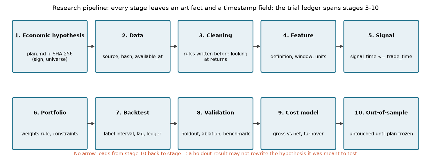
Figure 22-2: How search creates significance in a constructed world, and how a holdout distinguishes two worlds. Each of two worlds has 500 independent simulations, each with 200 stocks, a 120-month discovery sample, a 3-month embargo, and a 60-month holdout; the null-world seed is 20261006 and the alternative-world seed is 20261007 (the original chart’s shared title lists only 20261006, which must not be used to conflate the seeds). The left panel shows the null world (true IC is zero): blue is $|t|$ in the discovery sample for the single prespecified variant; orange is the maximum $|t|$ among 32 variants. The dashed line is 1.96, and the purple dotted line is the Bonferroni threshold of 3.16 for 32 tests. Interpretation: orange shifts to the right overall; 23.6% exceed 1.96, compared with 5.4% for blue. The right panel shows the holdout $t$-statistic of the best variant chosen in the discovery sample, aligned to its discovery sign: orange (null world) is centered around zero, while blue (true IC about 0.02) lies mostly to the right of zero. These are constructed data to illustrate a mechanism, not market evidence.

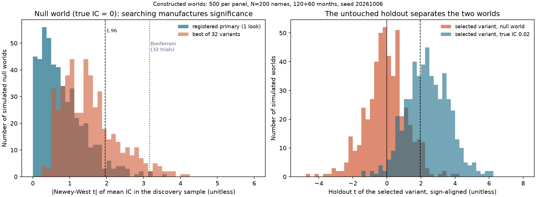
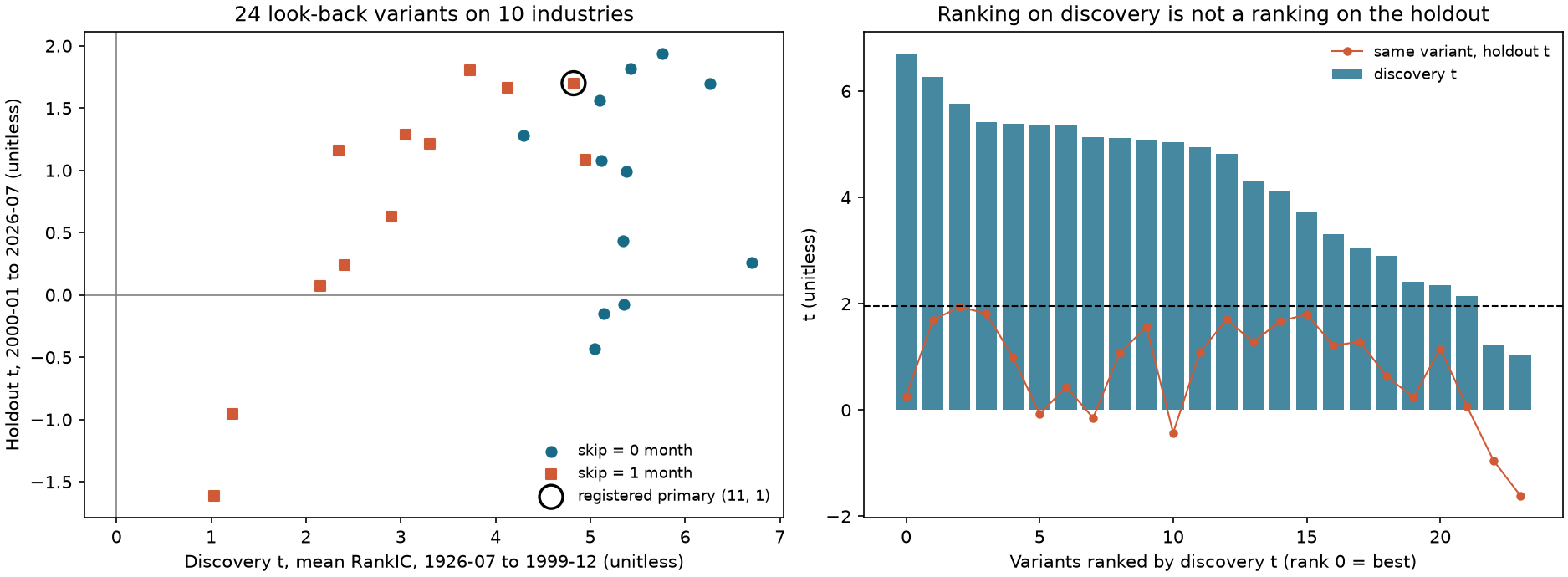
Figure 22-3: Twenty-four lookback-window variants for French industry momentum. In the left panel each point is a (lookback months, skip months) pair. The x-axis is the discovery-sample $t$ from 1926-07 through 1999-12; the y-axis is the holdout-sample $t$ from 2000-01 through 2026-07. The black circle marks the prespecified primary specification, (11, 1). In the right panel, variants are sorted by discovery $t$ from highest to lowest, and the orange line shows the holdout $t$ for the same variant. Interpretation: 22 of the 24 variants have $t>2$ in the discovery sample; none exceeds 2 in the holdout; the top-ranked variant, (1, 0), has a holdout $t$ of only 0.26. The sample consists of revised monthly returns for 10 industry portfolios, not executable trades.

11. Historical Market Example

Data. Use the French 10-industry value-weighted monthly returns frozen on 2026-10-05: source Ken French Data Library, 10 Industry Portfolios, ZIP SHA-256 ebd937a4b995d821867aeb956a96f09a666386f38fa82516b7d1767ee4a49ae5, processed CSV SHA-256 3b097d810c295d64eedfa1ece7067ff2a0707f5ca90e33935df9949251f70950, 1,202 months (1926-07 to 2026-08), in decimal monthly simple returns. Publicly downloadable does not mean freely redistributable. This chapter does not download new data.

Plan (frozen). Hypothesis: industries with higher past 12-1 returns have higher returns next month (positive sign). Signal: at month-end $s$, compound returns over the 11 months from $s-11$ through $s-1$, excluding the current month; label: simple return in the next month, $s+1$; cross-section: 10 industries; primary metric: the t-statistic of the mean monthly Spearman rank correlation (Rank IC) in the holdout sample (Newey–West lag 0); criterion: holdout $t\ge2.0$ and positive; cost assumption: 10 bp per unit of turnover, used only for the long-short portfolio demonstration; discovery sample through 1999-12, holdout sample from 2000-01 through 2026-07; trial budget of 24 variants (lookback 1–12 months, skip 0 or 1 month). The notes field says that this plan was written after reading the relevant literature and using the same data in earlier chapters; it is not a blind plan and was not externally registered.

Results. All numbers were produced by code/ch22_research_methodology.py and independently recomputed by qa/a5/claude/recompute/ch22_recompute.py (without importing course code, using a monthly loop and scipy.stats.spearmanr); the two agree.

Of the 24 variants, 22 have discovery-sample $t>2$ and none has holdout $t>2$. The ledger has 24 rows (the registered primary specification is the (11,1) row).

Apply the prespecified criterion. The primary specification’s holdout $t=1.70<2.0$, so the conclusion is “not supported.” The point estimate is positive (mean Rank IC 0.041); the difference between the discovery estimate (0.0688, standard error about 0.0143) and holdout estimate (0.0414, standard error about 0.0243) is about 0.027, with a standard error of about 0.028. The difference itself is not significant: the data neither prove that momentum “disappeared” after 2000 nor prove “no decay.” A permutation benchmark (randomly shuffling labels among the 10 industries each month 2,000 times while preserving each month’s label set) gives a one-sided p-value of 0.050, close to $1-\Phi(1.70)=0.045$, and adds no new information. These conclusions apply only to revised monthly returns for these 10 industry portfolios.

Multiple-testing adjustment. For the two-sided p-values of the 24 discovery-sample variants, the winner’s raw p-value is about $2\times10^{-11}$, with a Bonferroni-adjusted value of about $5\times10^{-10}$; Holm and BH are the same. It remains highly significant after adjustment. This shows that, under the approximate p-values and family definition used, the discovery-window tests still reject the null after adjustment; it does not identify why the holdout estimate is smaller. Multiple-testing adjustments control error rates for rejection decisions; they do not debias the selected effect size and cannot rule out the winner’s curse. Changes in the effect, selection bias, and sampling variation may all contribute; the difference above, 0.027 with standard error 0.028, does not establish decay. The lower holdout statistic also reflects estimation precision, so it cannot identify a cause.

Switch to a long-short portfolio and costs (demonstration). Each month, sort the 10 industries into five groups of two, go long the top group and short the bottom group, equal-weight each leg, for gross exposure of 2 and net exposure of 0. Turnover is the sum of absolute changes in target weights between adjacent months (buys and sells combined, not halved, ignoring drift). For the primary specification (11,1), the discovery-sample gross mean is 0.561% per month ($t=3.69$), mean turnover is 0.861, and net return at 10 bp per unit is 0.475%; the holdout gross mean is 0.403% ($t=1.21$), turnover is 1.019, and net return is 0.301%. For the discovery-sample winner (1,0), the discovery gross mean is 0.861% ($t=6.33$), the holdout gross mean is 0.405% ($t=1.25$), turnover is 3.056, and net return is 0.099% per month: turnover is three times higher and costs consume about three-quarters of the gross return. The 10 bp is an assumption, and industry portfolios are not executable trade series; the net returns here illustrate only the direction and relative size of gross returns and costs.

What this example does and does not show. It demonstrates that the registered primary specification, the discovery-sample winner, and the holdout sample can lead to very different conclusions; “not supported under the criterion” is not the same as “the estimate is significantly zero.” It does not prove that industry momentum does not exist, validate any conclusion in Chapter 25, or provide an independent test of 12-1 momentum: the holdout is not pristine, the author has read the momentum literature and used these data in earlier chapters, the cross-section has only 10 assets, and the data are revised historical values.

12. Common Errors

Error 1: Report only the best of $N$ variants. In a null world, the probability that the maximum $|z|$ among 20 independent variants exceeds 1.96 is $1-0.95^{20}=0.642$.

import numpy as np

rng = np.random.default_rng(7)
z = rng.standard_normal((20000, 20))                       # 20 independent null z-statistics per "paper"
reported_best = (np.abs(z).max(axis=1) > 1.96).mean()      # report only the best of 20
single = (np.abs(z[:, 0]) > 1.96).mean()                   # report the one pre-committed test
bonferroni = (np.abs(z).max(axis=1) > 3.0).mean()          # hurdle for 20 looks: z = 3.02 two-sided at 5%
assert abs(reported_best - (1 - 0.95**20)) < 0.015 and abs(single - 0.05) < 0.01 and bonferroni < 0.06
print(round(reported_best, 3), round(single, 3), round(bonferroni, 3))

Fix: report all variants or register one variant and state the budget in the plan. If search is unavoidable, use a Bonferroni or Holm threshold.

Error 2: Change the criterion after seeing results. The hash in Section 8.3 shows that changing one character in the criterion changes the entire hash. Fix: put the criterion in the plan and hash it; if a change is necessary, create a new version and record in the ledger and log that it was “changed after seeing the holdout result.”

Error 3: Repeatedly select using the holdout. If you evaluate 10 independent variants on the holdout and choose the best, the null-world probability of at least one “significant” result is $1-0.95^{10}=0.401$; the holdout has become a second discovery sample. Fix: evaluate only the single specification (or a small, explicitly counted number) selected in the discovery sample. Figure 22-3 calculates holdout $t$-statistics for all 24 variants to illustrate the chart; this is for teaching only. In real research it would amount to 24 holdout evaluations. The table in Section 11 still applies the criterion only to the registered primary specification and states this limitation explicitly.

Error 4: Use future data in standardization or winsorization parameters. Full-sample standardization of a time series makes early signals depend on later data.

import numpy as np

x = np.array([0.5, -0.2, 0.1, 0.4, -0.1, 3.0])        # pretend x[5] arrives later
full = (x - x.mean()) / x.std(ddof=0)                  # full-sample: uses the future
causal = np.array([(x[: i + 1] - x[: i + 1].mean())[-1] / (x[: i + 1].std(ddof=0) or 1.0) for i in range(len(x))])
x2 = x.copy(); x2[5] = -3.0                            # the future value changes ...
full2 = (x2 - x2.mean()) / x2.std(ddof=0)
causal2 = np.array([(x2[: i + 1] - x2[: i + 1].mean())[-1] / (x2[: i + 1].std(ddof=0) or 1.0) for i in range(len(x2))])
assert not np.allclose(full[:5], full2[:5])            # ... and rewrites earlier "signals"
assert np.allclose(causal[:5], causal2[:5])            # expanding-window version does not
print(np.round(full[0], 3), np.round(full2[0], 3))

Cross-sectional standardization across all stocks on the same day is not this error, because all the same-date data are available before signal_time; Chapter 28 distinguishes the two cases.

Error 5: Count only “successful” trials. The ledger must include abandoned and undefined attempts (n_trials is 6 in the second code sample in Section 9). Counting only successes is equivalent to reducing $M$ to the most favorable number.

Error 6: Naive $t$-statistics with overlapping labels. Three-month labels make the IC series correlated across adjacent months. In the null world, the standard deviation of $t$ for the three-month-label variant is 1.26 (1.04 for the one-month-label variant). Even with Newey–West lag 2, the rejection rate for $|t|>1.96$ on three-month labels is 11.8%, above the nominal 5%. In a finite sample, Newey–West underestimates variance. Fix: use a longer lag, nonoverlapping sampling, or calibrate the threshold separately for each $h$; Chapter 23 explains this in detail.

Error 7: Selection favors the statistic with the most biased standard error. In the same null world, the selected “best variant” has a 4.6% rate of holdout $t>1.96$ (aligned to the discovery sign), not 2.5%. Of the selected variants, 61.8% use three-month labels even though they make up only half of the variants. Their null $t$-statistics have higher variance, making them more likely to become the maximum; their holdout statistics also have higher variance. Selection favors the class with underestimated standard errors.

13. Quant Research Application: Compare an A Priori Fixed Plan with Post Hoc Mining for the Same Value Hypothesis

This section compares the value-hypothesis plan from Section 8.3 with a “mining version” on the same constructed data. The data are for teaching: 200 stocks, a 120-month discovery sample, a 3-month embargo, and a 60-month holdout. The feature is heavy-tailed monthly data (Student-$t$ with 4 degrees of freedom, variance-normalized) with autocorrelation 0.9, representing book-to-market ranks; next-period return equals $\text{slope}\times$ feature plus heavy-tailed noise (monthly standard deviation 0.08). The slope is 0 in the null world and 0.0016 in the alternative world, corresponding to population IC of about 0.020. The two worlds are otherwise identical. Each world is simulated 500 times.

Path A (a priori fixed specification): evaluate only variant 0 in the frozen plan (rank transform, lag 0, one-month label), and decide under the criterion. In the simulation, each month’s statistic is the “Pearson correlation between the rank-transformed signal and raw returns” (for vectorization, returns are not ranked), so it differs from Chapter 23’s Rank IC, which ranks both sides. Other variants use “the Pearson correlation between the transformed signal and raw returns,” consistent with the plan’s primary-metric wording. The real-data analysis in Section 11 uses Spearman Rank IC, ranking both sides. Path B (post hoc mining): evaluate 32 variants (rank/raw value/1% winsorization/5% winsorization × signal lags of 0–3 months × label horizons of 1 or 3 months), select the one with the largest discovery-sample $|t|$, and evaluate it on the holdout.

Interpretation. In the null world, Path B raises the false-positive rate from 5.4% to 23.6%, not to $1-0.95^{32}=81\%$: the variants are correlated. Matching the mean maximum discovery-sample $|t|$ of 1.53 implies about 4.6 effective independent trials, not 32. Using the Bonferroni threshold of 3.16 for the actual 32 attempts, the rejection rate in these 500 null-world simulations is 3.6%. This is not a general FWER guarantee: the union bound requires every marginal p-value to be valid, and the Newey–West approximate test may be miscalibrated here because the labels overlap. The 4.6 obtained by matching the mean maximum absolute statistic matches one moment and does not identify a tail threshold; Chapter 23 explains the Newey–West truncation and kernel-weight issue. In the alternative world, the power of Path A is 82.6%, while the holdout confirmation rate after selection on Path B is not much higher than A (61.8% versus 57.6%): search brings no reliable extra benefit, only more opportunities for false reporting. The holdout has only 60 months, so even when the signal is real, only about six in ten pass in the alternative world. This is a power issue, not a failure of the method.

Implication for Project 4: before a multifactor project starts, write a frozen plan containing at least the twelve items in Section 5, and specify the ledger format, embargo rule, and one-time holdout evaluation. Without this plan, no “significant” result from Project 4 can go into the conclusion. Chapter 28 will make preprocessing, combination, and constraints separate steps in the plan. The same applies to the pair screening in Project 5: the ledger must record how many cointegration tests were run during training (see the preparation layer at projects/project05/preparation/).

Benchmark and falsification condition: use equal-weight holdings (no signal) and a permutation benchmark; write before running that “the hypothesis is not supported if holdout $t<2.0$ or the sign is negative.”

14. Chapter Summary

This chapter divides a factor study into ten stages, each leaving an inspectable record. Four relationships matter. First, a frozen plan constrains choices that can be fixed before seeing results, while the ledger records every attempt whose result was read. Second, independent and well-calibrated tests give $1-(1-\alpha)^M$. With valid marginal p-values, Bonferroni and Holm control FWER without independence, while BH additionally requires independence or suitable positive dependence. In the particular constructed example, the mean maximum absolute statistic among 32 variants matches about 4.6 independent trials. This describes one moment; it cannot replace the actual family size or guarantee a tail threshold. Third, a holdout separates selection and evaluation. Avoiding repeated access and imposing an embargo reduce label leakage but do not automatically make financial data independent of the selection process; inference still requires checking dependence and marginal p-value calibration. Fourth, retain results that fail the prespecified criterion: the industry primary specification has holdout $t=1.70$, below the 2.0 threshold. None of these steps automatically establishes profitability after costs.

Limits: a local hash is not preregistration; the French industry data are revised historical data and have been used in earlier chapters; a cross-section of 10 assets has low testing power; costs are assumed values; and the chapter is a methodological demonstration, not an empirical verdict on any factor.

15. Exercises

22-E01 (Conceptual) What can a local freeze and an external preregistration each prove, and what can neither prove? If a colleague asks, “Does your hash timestamp predate the data?”, how should you answer?

22-E02 (Conceptual) Give an example of financial research with one regression and a hypothesis held in advance that still has forking paths. Identify the decision points.

22-E03 (By hand) For 20 independent tests at level $\alpha=1\%$, what is the family-wise error rate? What single-test level gives exactly 1% FWER (Šidák)? How far is it from Bonferroni?

22-E04 (By hand) Let $p=(0.002,\,0.011,\,0.020,\,0.040,\,0.300)$, $M=5$, and $\alpha=5\%$. Calculate the Bonferroni, Holm, and BH adjusted p-values, and list the tests that pass under each method.

22-E05 (Derivation) Use $\max(Z_1,Z_2)=\tfrac{Z_1+Z_2}2+\tfrac{|Z_1-Z_2|}2$ to derive $\mathbb E[\max(Z_1,Z_2)]=1/\sqrt\pi$. Explain why the DSR approximation is inaccurate at $N=2$.

22-E06 (Interpretation) In the null world, 32 variants have a mean maximum $|t|$ of 1.53, corresponding to about 4.6 effective independent trials. Explain what “effective number of independent trials” means. Compare Bonferroni using the actual $M=32$ with replacing that count by $M=4.6$: what conditions, power costs, or tail-error risks apply to each? Do both approaches necessarily contain an error in principle?

22-E07 (By hand) On a holdout sample, you evaluate 10 mutually independent null variants and report the best one. What is the probability that at least one has $|z|>1.96$? What does this imply for the rule “evaluate only once on the holdout”?

22-E08 (By hand) A long-short strategy has $T=60$ months and an estimated monthly Sharpe of 0.20. Calculate $t$, annualized Sharpe, and the two-sided p-value (normal approximation). If it is entered in a ledger with five variants, does it pass 5% after Bonferroni?

22-R01 (Ledger diagnosis, further practice) For the five-row ledger in Section 5.1, give the raw p-value vector used for the family, the Holm sorting multipliers, and the IDs rejected by each method at 5%. If you change the label horizon to the best value after H01, can that evaluation still be called an unexposed holdout? Could a file hash change the answer?

16. Programming Exercises

22-P01 Write your own ResearchPlan for any hypothesis, freeze it, and save it as JSON. Then change one field and verify that the hash differs; assert that overlapping discovery and holdout windows raise an error. Acceptance: all three assertions pass.

22-P02 Use a ledger to record eight variants, including one undefined result. Calculate two-sided p-values, use pad_untested_attempts to bring the full-ledger family size to $M=8$, and output a table of the three adjusted p-values. Acceptance: n_trials==8, family size is 8, and Bonferroni $\ge$ Holm $\ge$ BH for every test.

22-P03 Simulate 32 null $z$-statistics with an equicorrelation of 0.8. Across 20,000 simulations, calculate the mean maximum $|z|$ and the share exceeding 1.96, then use numerical integration to infer the equivalent number of independent trials. Acceptance: mean near 1.65 and equivalent number between 5 and 7.

17. Challenge Problems

22-C01 (Proof) Prove $\mathrm{FDR}\le\mathrm{FWER}$ and give a strict example with $\mathrm{FDR}<\mathrm{FWER}$ (specify the values of $V$ and $R$). Additional prerequisite: expectation and conditional probability. Grading: proof 40 points, example 40 points, practical interpretation 20 points.

22-C02 (Open-ended) Write a complete frozen plan for 12-1 momentum in Chapter 25: fill in all twelve items, specify ledger fields and embargo rules, describe the one-time holdout process, and list at least three concrete numerical outcomes that would lead you to conclude that the hypothesis is “not supported.” Grading: plan completeness 30 points, falsifiability of criteria 30 points, limitations for data repeatedly analyzed by others 20 points, cost and benchmark design 20 points.

18. Complete Solutions and Reference Implementations

22-E01 A local freeze binds normalized JSON to a digest. Under collision-resistance and related cryptographic assumptions, matching a trusted saved digest supports identity with the reference content. It does not prove that the file was never changed and later restored, or establish when it was written. A file and digest that can both be replaced do not establish their own trustworthy history. The local clock can be altered and cannot show that the plan preceded exposure. An external registry holds content or a digest with a third-party timestamp, providing evidence of registration chronology; prior data exposure must still be logged. Answer the colleague: “The current content can be compared with a trusted saved digest. The local time is not external evidence of chronology. These data were used before, so this is a process demonstration.”

22-E02 Example: study whether returns over the past 12 months predict returns next month. You hold the hypothesis in advance and run only one regression, but before seeing the results you did not fix whether to remove low-priced stocks, use value weights, exclude financial stocks, or choose the sample start. If the effect appears mainly among small-cap stocks, you can find a reasonable rationale for “exclude microcaps”; if it appears among large-cap stocks, you can find a rationale for “use value weights.” Regardless of how many regressions you actually ran, these data-dependent choices are forking paths.

22-E03 $\mathrm{FWER}=1-0.99^{20}=0.1821$. The Šidák single-test level is $1-(0.99)^{1/20}$: $\ln0.99=-0.0100503$, divided by 20 gives $-0.00050251$, and exponentiating gives $0.99949762$, so the complement is $0.00050238$. Bonferroni is $0.01/20=0.0005$. The difference is $2.4\times10^{-6}$, or about 0.5% relatively: Šidák is slightly more permissive, and the two are nearly identical in this range.

22-E04 $M=5$, with p-values already sorted in ascending order. Bonferroni $5p$ gives $0.010,\ 0.055,\ 0.100,\ 0.200,\ 1.000$; only the first ($p=0.002$) passes at 5%. Holm multipliers $5,4,3,2,1$ give $0.010,\ 0.044,\ 0.060,\ 0.080,\ 0.300$, already monotone; the first and second ($p=0.002,\,0.011$) pass. BH gives $p\cdot5/\text{rank}$: $0.010,\ 0.0275,\ 0.0333,\ 0.050,\ 0.300$. Taking the cumulative minimum from the end leaves these values; the first four pass at $\le0.05$ (the fourth is exactly 0.05 and counts as passing). In total, Bonferroni rejects 1, Holm 2, and BH 4; the more permissive error-rate definition allows more rejections.

22-E05 Both $Z_1+Z_2$ and $Z_1-Z_2$ are centered normal variables, and the expectation of the first term is 0. Let $W=Z_1-Z_2=\sqrt2\,G$, where $G\sim N(0,1)$. Then $\mathbb E|G|=\sqrt{2/\pi}$, so $\mathbb E|W|=\sqrt2\sqrt{2/\pi}=2/\sqrt\pi$ and $\mathbb E[\max]=\tfrac12\cdot2/\sqrt\pi=1/\sqrt\pi=0.5642$. The approximation gives 0.520, an underestimate of 7.9%. The authors call it a large-$N$ approximation. At $N=2$, $\Phi^{-1}(1-1/N)=\Phi^{-1}(0.5)=0$; the second term is $\Phi^{-1}(1-1/(2e))=\Phi^{-1}(0.816)=0.90$. Weighting it by $0.5772$ gives $0.52$. The asymptotic expansion from extreme-value theory has non-negligible error at small $N$. (Readers can check with expected_max_standard_normal(2).)

22-E06 Here $N_{\mathrm{eff}}$ is defined by matching one moment: the expected maximum of $N_{\mathrm{eff}}$ independent $|N(0,1)|$ variables equals the observed mean of 1.53 in this constructed example. Numerical inversion gives about 4.6. This does not mean that the full maximum distributions are the same, and it gives no tail-probability or FWER guarantee. Bonferroni with the actual $M=32$ uses a threshold of about 3.16 and controls FWER by the union bound when marginal p-values are valid; independence is not required, though power may be lower. The 3.6% rejection rate in this null world and 65.8% in the alternative world are only results from this simulation; the overlapping-label/Newey–West calibration limitations remain. Replacing 32 with 4.6 would relax the threshold to about 2.55, but matching a mean does not establish that this threshold controls 5% FWER. Nor can it provide such a guarantee when the dependence structure is unknown or marginal p-values are invalid. Keep the full-ledger adjustment, or rerun the entire selection process under a resampling design that preserves both the null and dependence structure and estimates the tail of the maximum distribution; the validity of the resampling design must itself be justified.

22-E07 $1-0.95^{10}=0.4013$. Evaluating 10 variants on the holdout and selecting the best gives a Type I error rate of about 40%; the holdout has become a second discovery sample. The rule “evaluate only once on the holdout” means evaluating only the specification selected after freezing (or a small number that is explicitly counted).

22-E08 $t=0.20\sqrt{60}=1.549$; annualized Sharpe $0.20\sqrt{12}=0.693$; two-sided $p=2(1-\Phi(1.549))=0.121$. In a five-variant ledger, Bonferroni gives $p=\min(5\times0.121,1)=0.606$, which does not pass. Here, $t=\widehat{SR}_m\sqrt T$ assumes monthly returns are approximately independent and identically distributed.

22-R01 The family’s raw p-value vector is $(0.01,0.04,0.03,1,0.005)$. In ascending order the IDs are D05, D01, D03, D02, D04; Holm multipliers are $5,4,3,2,1$. The products are $0.025,0.04,0.09,0.08,1$, and the cumulative maxima are $0.025,0.04,0.09,0.09,1$. Mapping back to the original rows gives the values in Section 5.1. At $p_{\mathrm{adj}}\le0.05$, Bonferroni and Holm reject D01 and D05; BH rejects D01, D02, D03, and D05 (including equality). The BH FDR guarantee additionally requires independence or an applicable positive-dependence condition. Changing the horizon after H01 uses holdout information, so the data can no longer be called unexposed; a hash binds file contents but cannot undo the history of what was read.

22-P01 Reference Implementation

import dataclasses
import json
from datetime import datetime, timezone

import pytest

from quant_course.research_protocol import ResearchPlan, freeze_plan

plan = ResearchPlan(
    hypothesis="Higher past 12-1 return predicts higher next-month return (sign +)",
    universe="10 French industries", data_sources=("french_10_industries_monthly.csv",),
    discovery_start="1926-07", discovery_end="1999-12", holdout_start="2000-01", holdout_end="2026-07",
    signal_definition="12-1 compounded return", label_definition="next-month simple return",
    portfolio_rule="top 2 minus bottom 2, equal weight", benchmark="equal-weight 10 industries",
    primary_metric="t of mean RankIC in holdout", decision_rule="holdout t >= 2.0 and positive",
    cost_assumption="10 bp per unit traded", trial_budget=24,
)
clock = datetime(2026, 10, 6, 9, 0, tzinfo=timezone.utc)
first = freeze_plan(plan, now=clock)
second = freeze_plan(dataclasses.replace(plan, trial_budget=25), now=clock)
assert first.sha256 != second.sha256
saved = json.dumps({"sha256": first.sha256, "frozen_at_local": first.frozen_at_local}, indent=1)
assert json.loads(saved)["sha256"] == first.sha256
with pytest.raises(ValueError):
    dataclasses.replace(plan, holdout_start="1999-06")        # overlaps the discovery window

22-P02 Reference Implementation

import numpy as np
import pandas as pd
from scipy import stats

from quant_course.research_protocol import (
    TrialLedger, benjamini_hochberg_adjust, bonferroni_adjust, holm_adjust, pad_untested_attempts,
)

t_values = [2.8, 2.1, 1.7, 1.2, 0.9, 0.5, -0.4]
ledger = TrialLedger()
for i, value in enumerate(t_values):
    ledger.record({"variant": i}, metric=value, n_obs=120, status="primary" if i == 0 else "run")
ledger.record({"variant": 7}, metric=float("nan"), n_obs=0, status="abandoned", note="constant signal")
assert ledger.n_trials == 8
p = np.append(2 * stats.norm.sf(np.abs(np.array(t_values))), np.nan)          # the undefined attempt has no p-value
family = pad_untested_attempts(p[:-1], ledger.n_trials)                          # ... and enters the family as p = 1: M = 8
assert family.size == 8 and family[-1] == 1.0
table = pd.DataFrame({"t": t_values + [np.nan], "p": family, "bonf": bonferroni_adjust(family), "holm": holm_adjust(family),
                      "bh": benjamini_hochberg_adjust(family)})
assert (table["bonf"] >= table["holm"] - 1e-12).all() and (table["holm"] >= table["bh"] - 1e-12).all()
assert (table["bonf"].iloc[-1], table["holm"].iloc[-1], table["bh"].iloc[-1]) == (1.0, 1.0, 1.0)
print(table.round(4))

(The seven t-values plus one undefined attempt make eight ledger rows. Add the undefined attempt to the family as $p=1$, so the primary convention is $M=8$. Adjusting only the seven valid p-values ($M=7$) is a different convention and may be reported only as a sensitivity note.)

22-P03 Reference Implementation

import numpy as np
from scipy import integrate, optimize, stats


def mean_max_abs_normal(n):
    cdf = lambda x: 2 * stats.norm.cdf(x) - 1
    pdf = lambda x: 2 * stats.norm.pdf(x)
    return integrate.quad(lambda x: x * n * pdf(x) * cdf(x) ** (n - 1), 0, 12, limit=200)[0]


rng = np.random.default_rng(1)
m, rho, worlds = 32, 0.8, 20000
common = rng.standard_normal((worlds, 1))
z = np.sqrt(rho) * common + np.sqrt(1 - rho) * rng.standard_normal((worlds, m))
observed = np.abs(z).max(axis=1).mean()
n_eff = optimize.brentq(lambda n: mean_max_abs_normal(n) - observed, 1.0, 500.0)
assert 1.55 < observed < 1.75 and 5.0 < n_eff < 7.0
assert abs(mean_max_abs_normal(32) - 2.347) < 0.01
print(round(observed, 3), round(n_eff, 2), round((np.abs(z).max(axis=1) > 1.96).mean(), 3))

The output is approximately 1.648, 5.92, and 0.258: the maximum absolute value of 32 variants with correlation 0.8 matches about six independent trials on this one moment. Under the null, taking the maximum leads to rejection at 1.96 in 26% of cases, far below the 81% for independent tests.

22-C01 Let $V$ be the number of false rejections and $R$ the total number of rejections. If $V\ge1$, then $R\ge1$ and $V/R\le1$; if $V=0$, then $V/\max(R,1)=0$. Therefore, $V/\max(R,1)\le\mathbf 1\{V\ge1\}$. Taking expectations gives $\mathrm{FDR}\le\Pr(V\ge1)=\mathrm{FWER}$. For a strict example, let $M=10$, with $m_0=5$ true nulls and five false nulls that are almost surely rejected. If one true null is falsely rejected, then $V=1$, $R=6$, and $V/R=1/6<1$, while $\mathbf 1\{V\ge1\}=1$. If this occurs with positive probability, FDR is strictly lower than FWER. Meaning: FDR allows a few errors among many true discoveries and is more useful in exploration; a claim about a single factor calls for the stricter FWER. Grade the three parts as in the original.

22-C02 (Scoring Guide and Reference) A sample plan: hypothesis: “the higher the compounded return over the past 12-1 months, the higher the return next month (positive sign)”; state whether the stock universe includes small caps and financials; specify total-return price data and available_at; give discovery and holdout endpoints; signal: 12-1 (11-month window, skip 1 month); label: next month; portfolio: equal-weight decile long-short, rebalanced monthly; benchmarks: equal-weight and permutation; primary metric: holdout Rank IC $t$; criterion: prespecify holdout Rank IC $t\ge2.0$ with a positive sign as the sole primary confirmation; list after-cost portfolio results separately as secondary evaluation with risk constraints. If multiple metrics jointly confirm, state “all must pass” or a multiplicity-adjusted joint rejection rule before opening the holdout; do not select whichever is significant after the fact. Give a specific cost assumption in basis points; trial budget (for example, 12); ledger fields; embargo rule (one-month label, one-month embargo); and one-time holdout process. The following are illustrative constructed values, not estimates from the French history. Three outcomes that fail the primary hypothesis criterion are: mean holdout Rank IC 0.02 with $t=1.70$; mean $-0.01$ with $t=-2.3$ (wrong direction); and mean 0.001 with $t=0.1$ (insufficient precision). Separately, if a nonnegative mean net return was prespecified as an economic-feasibility gate, a net mean of $-0.002$ fails that secondary gate; it does not automatically overturn the sole IC statistical hypothesis if that passed. Report statistical confirmation and after-cost economic feasibility separately. A different study with net return as its primary hypothesis must fix its test and multiplicity rule before opening the holdout. State the limits: the data have been repeatedly used by others, the local hash is not external preregistration, and costs are assumptions. Grade the four parts as in the original. Acceptable variations in the twelve items and thresholds are fine if they are falsifiable and fixed before running.

19. Further Reading

• Must know: Harvey–Liu–Zhu working paper Sections 4.3–4.4 (definitions and examples of FWER, FDR, Bonferroni, and Holm); read the abstract and introduction first, then these sections. Purpose: understand why $t>2$ is no longer enough.
• Must know: Gelman–Loken, Sections 1.1–1.2 and 4.3, on forking paths and the limits of preregistration.
• Should know: the first half of Bailey–López de Prado’s Deflated Sharpe Ratio, Eq. (1) and Appendix A.1; read the full construction again in Chapter 32.
• Should know: the definition in Section 2 of Bailey et al.’s PBO paper, on overfitting in the selection process; used in Chapters 30–32.
• Advanced: the original papers by Holm (1979), Benjamini–Hochberg (1995), and Benjamini–Yekutieli (2001), to check the conclusions in Sections 6.3 and 6.4; these originals have not been read for this chapter.
• Optional: instructions from any public preregistration platform to learn how external timestamps work.

20. References

Citation keys and reading ranges are listed in source_notes.md.

• CH22_HLZ2014: Harvey, C. R., Liu, Y., Zhu, H. (2014). “… and the Cross-Section of Expected Returns.” NBER Working Paper 20592. Supports Sections 2, 5, 6.3, and 7; the 2016 RFS journal version has not been read.
• CH22_DSR2014: Bailey, D. H., López de Prado, M. (2014). “The Deflated Sharpe Ratio.” Authors’ 2014-07-31 preprint. Supports the equation in Section 6.5.
• CH22_PBO2015: Bailey, D. H., Borwein, J. M., López de Prado, M., Zhu, Q. J. (2015). “The Probability of Backtest Overfitting.” Authors’ preprint. Used only as a conceptual preview in Sections 5 and 19.
• CH22_GELMANLOKEN2013: Gelman, A., Loken, E. (2013). “The garden of forking paths.” Unpublished working paper. Supports Sections 2, 3, and 5.
• CH22_JT1993: Jegadeesh, N., Titman, S. (1993). “Returns to Buying Winners and Selling Losers.” Journal of Finance 48(1), printed pages 68–69; supports the Bonferroni discussion of 32 strategies in Section 7.
• FRENCH: Kenneth R. French Data Library, 10 Industry Portfolios (frozen snapshot and hash in Section 11 and data/manifests/french_industries_2026-10-05.json).