Project 2 Research Report: CAPM and Fama–French Factor Attribution
Reader note: The data version, values, negative results, and null results below are retained from the historical study. They are historical teaching material, not new market results from the current constructed-data run of the I3 reader notebook. The package’s default Project 2 notebook is a separate constructed-data demonstration: its three models use the same generated factor columns and are strictly nested. Its outputs are not the historical market results reported here. The data-authorization branch is skipped by default.
This project uses the Capital Asset Pricing Model (CAPM), the Fama–French Three-Factor Model (FF3), and the Fama–French Five-Factor Model (FF5). Ordinary Least Squares (OLS) estimates the coefficients; Heteroskedasticity and Autocorrelation Consistent (HAC) covariance estimation is used for inference; and confidence intervals (CIs) and the Holm step-down multiple-testing adjustment describe single-estimate uncertainty and adjustment across the stated test family, respectively. The theory and worked calculations are covered in Chapters 8 and 15.
Historical status of the original project: verified (this does not mean the market analysis was re-verified for this reader package); completed by the root author and independent reviewer. This report is based on the fixed configuration and frozen data manifest; the tables were calculated by a reproducible CLI.
Conclusions
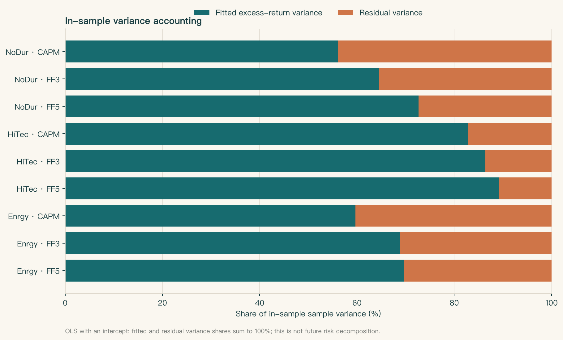
For the 120-month historical snapshot from January 2010 through December 2019, in-sample R² under FF5 is 0.727, 0.893, and 0.696 for NoDur, HiTec, and Enrgy, respectively; under CAPM it is 0.561, 0.829, and 0.597. This comparison has a higher in-sample fitted variance share under FF5, but this means only that the contemporaneously published factors provide a larger linear fit to the same historical returns.
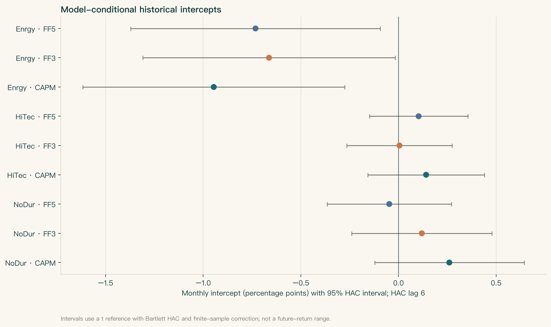
All six Alpha estimates for NoDur and HiTec have HAC 95% intervals that cross zero. All three Enrgy Alpha estimates are negative, and their individual HAC 6 intervals lie below zero. After Holm adjustment across the nine asset-by-model Alpha estimates shown in this report, the minimum p-value is 0.0549; none is below 0.05. This does not prove that energy portfolios will continue to underperform, and Alpha is not an asset attribute independent of the model. All negative and near-zero results are retained.
The study has no causal identification, historical point-in-time data, signal, order, or execution ledger. It does not test a trading advantage. Costs, financing, and borrowing are not applicable to these data; no after-cost strategy return or Alpha was calculated.
Research question, data, and timing
The questions are: What conditional relationships do the excess returns of three industry portfolios have with the same-month published spreads for the market, size, value, profitability, and investment factors? How do Beta, model-specific intercepts, R², and residuals change as factors are added? How sensitive are the results to the HAC bandwidth and fixed historical slices?
The assets are Non-Durables (NoDur), Hi-Tech (HiTec), and Energy (Enrgy) from Kenneth R. French’s U.S. 10 industry portfolios, using value-weighted monthly total returns with dividends. The French Data Library and methodology are described in the official library, industry portfolio description, FF3 description, and FF5 description. The original studies are Fama and French (1993) and (2015): 1993, 2015.
The inputs are the current release snapshot downloaded and frozen on 2026-10-05; both the FF3 and FF5 file headers identify the 202608 CRSP version. The data manifest records the ZIP, member CSV, processed CSV path, and SHA-256 for each of the three inputs. The CLI checked all hashes, ZIP CRCs, archive members, and byte identity with the saved original CSVs, then validated the actual input through the shared monthly reader. The project did not re-download, overwrite, or rebuild the production data.
French files are published in percent units; the frozen processed CSVs were divided by 100 once, and this project reads decimal returns without another conversion. The source missing-value sentinels −99.99 and −999 were converted to empty fields during preprocessing. Any missing or infinite selected value, missing month, duplicate month, or misalignment causes an error; gaps are neither filled nor compressed. The main sample is fixed at 2010-01 through 2019-12, with exactly 120 matching monthly PeriodIndex values for each asset and factor.
Official documentation states that, beginning with the January 2025 release, the library switched from the older CRSP FIZ format to CIZ Flat File Format 2.0, which uses a different monthly dividend-reinvestment timing convention. The source of the RF proxy also changed in June 2024 from Ibbotson Associates to the ICE BofA US 1-Month Treasury Bill Index. The current historical files are one revised snapshot, not a historical point-in-time (PIT) archive. A public download is not a general redistribution license; external use must retain Fama and French attribution and check the current terms.
Month labels identify return intervals. They do not provide historical event_time, available_at, signal_time, or trade_time. The manifest’s download date records when the current snapshot was obtained; it cannot establish what was knowable historically. There is no signal and no future-return label.
Model, inference, and interpretation
For asset i and month t, the target is y(i,t) = R(i,t) − RF(t), and the model is:
RF is subtracted once from the asset’s dividend-inclusive total return; Mkt-RF, SMB, HML, RMW, and CMA are published spreads and enter the right-hand side in their original form. CAPM uses Mkt-RF and RF from the FF3 file; FF3 and FF5 each use the full set of factors and RF from their corresponding official file. Units are decimal monthly returns. There is no inner join that drops months, no date shift, and no repeated percentage conversion.
OLS includes an intercept. Alpha is a conditional mean intercept for a particular sample and model benchmark; it changes when the factor set or sample changes. It is not a demonstrated pricing error, skill, or future return. Beta is a linear conditional loading given the other factors in the model. For example, Beta = 0.8 means that when a same-month factor spread rises by 1 percentage point, the fitted conditional mean excess return changes by about 0.8 percentage points. This is statistical co-movement, not causation. SMB is small minus big, HML is high minus low book-to-market, RMW is robust minus weak profitability, and CMA is conservative minus aggressive investment, using the published spreads. Portfolio Betas should not be over-interpreted as firm-level mechanisms.
The main results use HAC standard errors with a Bartlett kernel, six monthly observation-row lags, a finite-sample correction, and a t reference distribution. Standard errors, intervals, and p-values for all coefficients were also calculated with 3, 6, and 12 monthly lags. Changing the HAC bandwidth does not change the OLS point estimates; it changes inference. HAC does not add omitted variables, resolve endogeneity, remove structural change, or validate error assumptions. Small-sample intervals and p-values are approximations that depend on assumptions.
R² is the in-sample proportion of squared error reduced relative to the mean benchmark; adjusted R² accounts for degrees of freedom. With an intercept, the OLS residual sample mean is close to zero. We checked that, for the same 120-month target and ddof=1, the variances satisfy Var(y)=Var(fitted)+Var(residual). This is an in-sample accounting identity for the OLS projection, not a causal decomposition or evidence of future predictive ability. Because factors may be correlated, marginal Betas are not converted into independent, additive factor risk shares.
The nine-test Alpha family consists of three fixed assets crossed with three fixed models. The report gives nominal HAC p-values and Holm step-down adjusted values. Holm covers only these nine displayed intercepts, not other model searches, factor definitions, or window choices. Beta intervals are pointwise and do not adjust for the full specification search.
The OLS and four-month hand calculation examples are in Chapter 15, Sections 6 and 8; the step-by-step numerical Bartlett HAC sandwich-matrix example is in Section 6.4 of that chapter. The 95% intervals in the tables are pointwise; Holm adjustment applies only to the p-values of the nine intercepts, so these intervals are not simultaneous confidence intervals.
Nine full-sample empirical results
Alpha and its confidence interval are in percentage points per month; Beta is dimensionless, with its HAC 6 95% interval in brackets. A dash means the factor is not included in that model; it does not mean the estimated value is zero. Exact results, t-statistics, and p-values for every coefficient are in the HAC 6 coefficient CSV (historical external evidence/data not bundled).
NoDur: Non-Durables
| Model | Alpha (% / month) [95% CI] | Alpha p / Holm p | Mkt-RF | SMB | HML | RMW | CMA | R² / adjusted R² |
|---|---|---|---|---|---|---|---|---|
| CAPM | 0.2603 [−0.1223, 0.6429] | 0.1804 / 1.0000 | 0.646 [0.539, 0.752] | — | — | — | — | 0.561 / 0.557 |
| FF3 | 0.1195 [−0.2392, 0.4782] | 0.5108 / 1.0000 | 0.747 [0.646, 0.848] | −0.424 [−0.611, −0.237] | −0.117 [−0.304, 0.070] | — | — | 0.645 / 0.636 |
| FF5 | −0.0472 [−0.3653, 0.2710] | 0.7695 / 1.0000 | 0.812 [0.723, 0.902] | −0.296 [−0.521, −0.071] | −0.251 [−0.411, −0.090] | 0.526 [0.291, 0.762] | 0.481 [0.204, 0.759] | 0.727 / 0.715 |
HiTec: Hi-Tech
| Model | Alpha (% / month) [95% CI] | Alpha p / Holm p | Mkt-RF | SMB | HML | RMW | CMA | R² / adjusted R² |
|---|---|---|---|---|---|---|---|---|
| CAPM | 0.1414 [−0.1568, 0.4396] | 0.3496 / 1.0000 | 1.097 [1.022, 1.171] | — | — | — | — | 0.829 / 0.827 |
| FF3 | 0.0051 [−0.2643, 0.2746] | 0.9701 / 1.0000 | 1.158 [1.075, 1.242] | −0.155 [−0.306, −0.004] | −0.337 [−0.485, −0.189] | — | — | 0.864 / 0.861 |
| FF5 | 0.1032 [−0.1486, 0.3550] | 0.4185 / 1.0000 | 1.126 [1.019, 1.233] | −0.158 [−0.320, 0.003] | −0.050 [−0.199, 0.099] | 0.021 [−0.257, 0.299] | −0.668 [−0.962, −0.374] | 0.893 / 0.888 |
Enrgy: Energy
| Model | Alpha (% / month) [95% CI] | Alpha p / Holm p | Mkt-RF | SMB | HML | RMW | CMA | R² / adjusted R² |
|---|---|---|---|---|---|---|---|---|
| CAPM | −0.9459 [−1.6167, −0.2752] | 0.0061 / 0.0549 | 1.195 [1.081, 1.309] | — | — | — | — | 0.597 / 0.593 |
| FF3 | −0.6629 [−1.3091, −0.0167] | 0.0444 / 0.3111 | 1.065 [0.936, 1.195] | 0.332 [0.078, 0.585] | 0.692 [0.375, 1.008] | — | — | 0.688 / 0.680 |
| FF5 | −0.7323 [−1.3707, −0.0939] | 0.0249 / 0.1995 | 1.090 [0.922, 1.258] | 0.286 [0.049, 0.524] | 0.452 [0.046, 0.858] | −0.091 [−0.564, 0.381] | 0.508 [−0.065, 1.082] | 0.696 / 0.683 |
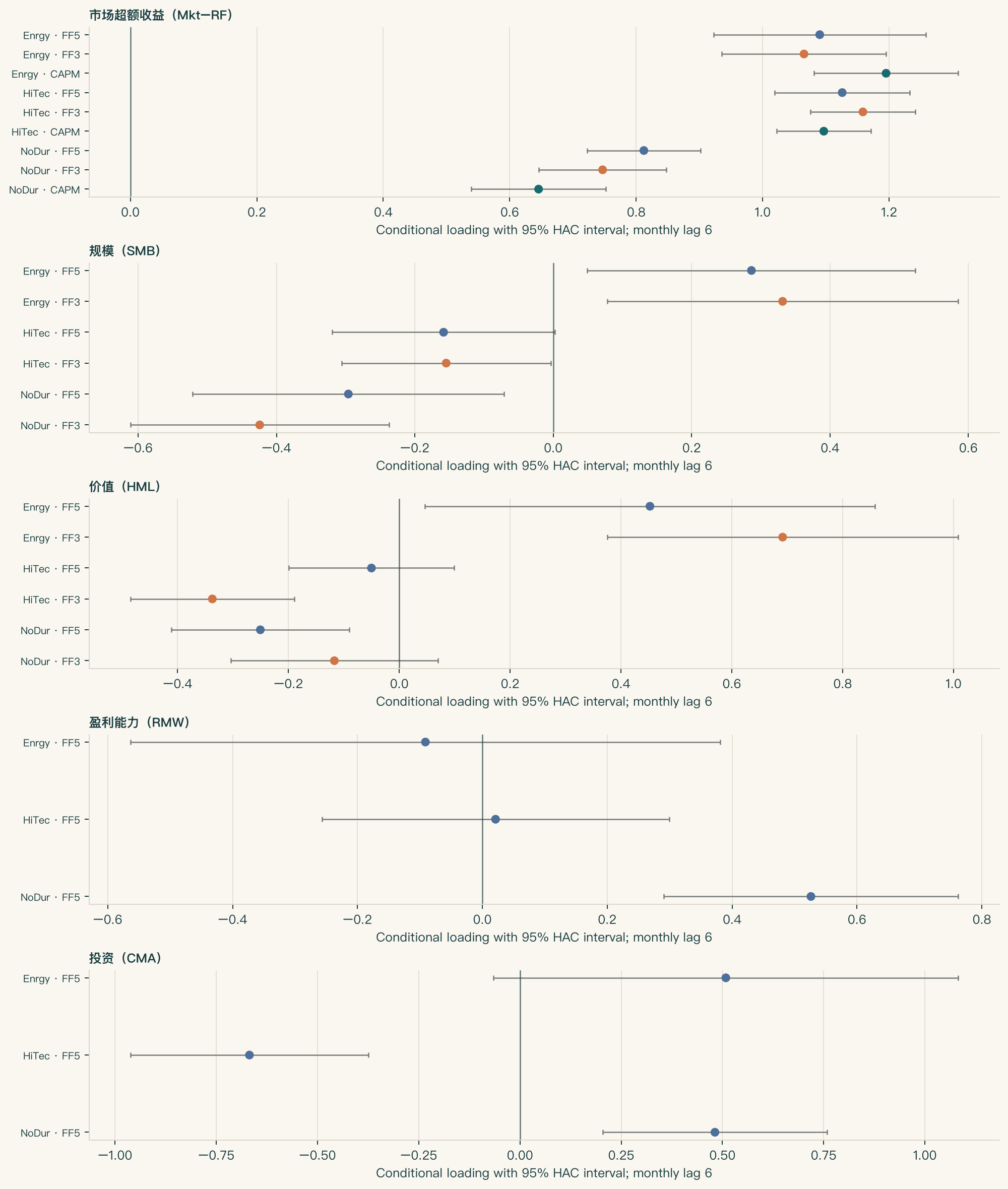
HiTec’s market Beta is above 1; all three assets have positive market Betas. Other loading signs depend on the industry and benchmark. The HiTec FF5 SMB interval narrowly crosses zero; the Enrgy FF5 RMW and CMA intervals cross zero; and the NoDur FF3 HML interval crosses zero. All are retained. The three energy intercepts have individual HAC 6 intervals below zero, but none reaches the 5% threshold after the nine-test Holm adjustment. The intervals for the other six intercepts cross zero; HiTec FF3 is close to zero at 0.0051% per month.
HAC bandwidth sensitivity
The table gives 95% intervals for the nine Alpha estimates at each bandwidth, in percentage points per month. Full point estimates, standard errors, t-statistics, p-values, and intervals for all Alpha and Beta coefficients under HAC 3/6/12 are in the complete sensitivity CSV (historical external evidence/data not bundled).
| Asset | Model | HAC 3 | HAC 6 | HAC 12 |
|---|---|---|---|---|
| NoDur | CAPM | [−0.1276, 0.6482] | [−0.1223, 0.6429] | [−0.1532, 0.6738] |
| NoDur | FF3 | [−0.2285, 0.4674] | [−0.2392, 0.4782] | [−0.2836, 0.5226] |
| NoDur | FF5 | [−0.3453, 0.2510] | [−0.3653, 0.2710] | [−0.4124, 0.3181] |
| HiTec | CAPM | [−0.1620, 0.4448] | [−0.1568, 0.4396] | [−0.1744, 0.4572] |
| HiTec | FF3 | [−0.2846, 0.2948] | [−0.2643, 0.2746] | [−0.2589, 0.2691] |
| HiTec | FF5 | [−0.1768, 0.3832] | [−0.1486, 0.3550] | [−0.1449, 0.3513] |
| Enrgy | CAPM | [−1.6232, −0.2687] | [−1.6167, −0.2752] | [−1.5996, −0.2923] |
| Enrgy | FF3 | [−1.2950, −0.0308] | [−1.3091, −0.0167] | [−1.3154, −0.0104] |
| Enrgy | FF5 | [−1.3793, −0.0854] | [−1.3707, −0.0939] | [−1.3766, −0.0880] |
The three individual energy intervals remain below zero at all three HAC bandwidths, but these are not three independent batches of evidence. The displayed nine-test Holm adjustment uses HAC 6 and leaves no intercept significant at 5%; separate Holm adjustments at HAC 3 or HAC 12 are not claimed. Changing the bandwidth affects inference, not the Beta or Alpha point estimates.
Fit, residuals, and risk decomposition
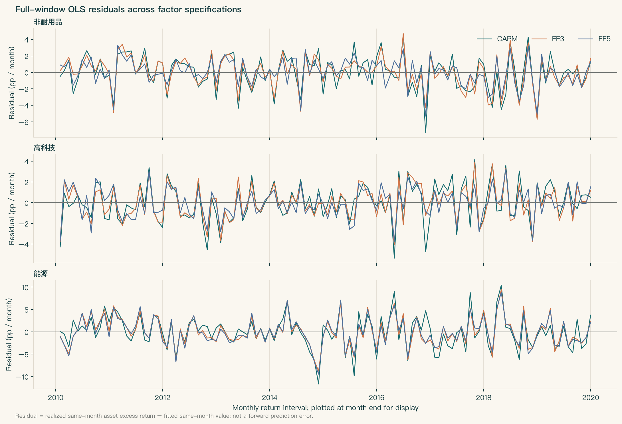
Residual metrics are in percentage points per month; Lag-1 is the sample correlation between adjacent months. A mean near zero is an in-sample property of OLS with an intercept. Monthly targets, fitted values, and residuals are in the residual CSV (historical external evidence/data not bundled).
| Asset | Model | R² | Fitted variance share | Residual variance share | Residual SD | RMSE | MAE | Maximum absolute value | Lag-1 |
|---|---|---|---|---|---|---|---|---|---|
| NoDur | CAPM | 0.561 | 56.080% | 43.920% | 2.137 | 2.128 | 1.686 | 7.278 | −0.063 |
| NoDur | FF3 | 0.645 | 64.496% | 35.504% | 1.921 | 1.913 | 1.455 | 5.696 | −0.072 |
| NoDur | FF5 | 0.727 | 72.651% | 27.349% | 1.686 | 1.679 | 1.297 | 5.314 | −0.200 |
| HiTec | CAPM | 0.829 | 82.879% | 17.121% | 1.864 | 1.856 | 1.494 | 5.360 | −0.146 |
| HiTec | FF3 | 0.864 | 86.407% | 13.593% | 1.661 | 1.654 | 1.364 | 4.075 | −0.180 |
| HiTec | FF5 | 0.893 | 89.273% | 10.727% | 1.475 | 1.469 | 1.197 | 3.758 | −0.178 |
| Enrgy | CAPM | 0.597 | 59.670% | 40.330% | 3.674 | 3.659 | 2.794 | 11.684 | 0.009 |
| Enrgy | FF3 | 0.688 | 68.799% | 31.201% | 3.232 | 3.218 | 2.541 | 9.437 | 0.043 |
| Enrgy | FF5 | 0.696 | 69.598% | 30.402% | 3.190 | 3.177 | 2.486 | 9.482 | 0.075 |
R² corresponds to the fitted variance share and describes in-sample variance accounting. It does not show that future volatility will fall, that factor risk is tradable, or that RMW/CMA alone caused the FF5 improvement.
Figure descriptions:
- Alpha figure: The x-axis is monthly Alpha (percentage points per month); the y-axis identifies each asset-by-model estimate; points show estimates, horizontal lines show HAC 6 95% intervals, and the vertical line marks zero.
- Loading figure: The five panels show market, size, value, profitability, and investment. The x-axis is conditional Beta; the y-axis identifies each asset-by-model that includes the factor; lines show HAC 6 intervals. Factors not included in a model are not shown as zero.
- Variance figure: The x-axis is each model’s fitted and residual shares of excess-return variance for the same sample, as percentages; the y-axis identifies the nine models. Teal is the fitted component and orange the residual component; each bar sums to 100%.
- Residual figure: The x-axis is the monthly return interval, labeled at month-end for plotting; the y-axis is realized same-month excess return less its fitted value, in percentage points per month. The three panels are the three industries, and colors distinguish CAPM, FF3, and FF5. These are not future forecast errors.
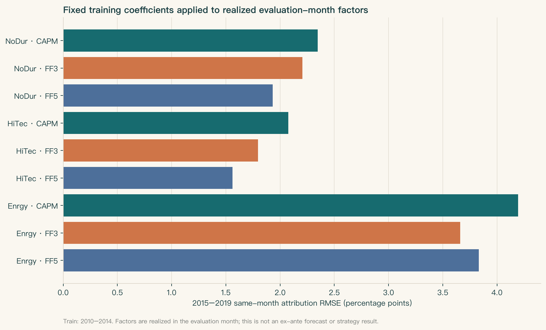
- Chronological attribution-error figure: The x-axis is 2015–2019 same-month attribution RMSE, in percentage points; the y-axis identifies each asset-by-model. Horizontal bars show RMSE after coefficients estimated on 2010–2014 are applied to factors realized during each evaluation month. This is not an ex ante forecast or strategy result.
FF3 and FF5 factor differences
The main results retain the corresponding official series. Differences in common columns over 2010–2019 are:
| Field | Maximum absolute difference (decimal / month) | Number of different months |
|---|---|---|
| Mkt-RF | 0.0003 | 40 / 120 |
| SMB | 0.0137 | 119 / 120 |
| HML | 0 | 0 / 120 |
| RF | 0 | 0 / 120 |
Both original files identify the 202608 CRSP version. Locally, each was converted from percent to decimal once; the selected HML and RF series match exactly, while Mkt-RF and SMB differ. The difference in SMB construction has an official explanation: the FF3 construction description uses six size-by-book-to-market portfolios, while the FF5 construction description averages three size spreads formed on book-to-market, profitability, and investment. Thus, not all SMB construction differences can be called unknown. This project has not reproduced the month-by-month differences from the underlying portfolios. The specific cause of the Mkt-RF file-value difference is also unknown; we do not guess that it is rounding, revision, or a release error. Because the common-factor values are not identical, the official FF3 and FF5 models are not strictly nested. We do not run a nested-model F-test or attribute the full R² increase to the added RMW/CMA factors. To isolate their contribution, hold the same baseline factors fixed and then add RMW/CMA, labeling the result a custom specification and a new study.
Chronological attribution check
Intercepts estimated on 2010–2014 compared with the full-window intercepts (percentage points per month):
| Asset | Model | Training Alpha | Full-window Alpha | Full window minus training |
|---|---|---|---|---|
| NoDur | CAPM | 0.525 | 0.260 | −0.264 |
| NoDur | FF3 | 0.379 | 0.119 | −0.260 |
| NoDur | FF5 | 0.144 | −0.047 | −0.191 |
| HiTec | CAPM | −0.147 | 0.141 | 0.288 |
| HiTec | FF3 | −0.252 | 0.005 | 0.257 |
| HiTec | FF5 | −0.098 | 0.103 | 0.201 |
| Enrgy | CAPM | −0.752 | −0.946 | −0.194 |
| Enrgy | FF3 | −0.617 | −0.663 | −0.046 |
| Enrgy | FF5 | −0.585 | −0.732 | −0.148 |
Applying the training estimates to realized same-month factors in 2015–2019 gives these error statistics (percentage points per month):
| Asset | Model | Mean error | RMSE | MAE | Maximum absolute error |
|---|---|---|---|---|---|
| NoDur | CAPM | −0.541 | 2.347 | 1.747 | 7.570 |
| NoDur | FF3 | −0.666 | 2.205 | 1.656 | 5.800 |
| NoDur | FF5 | −0.459 | 1.932 | 1.516 | 5.293 |
| HiTec | CAPM | 0.601 | 2.075 | 1.682 | 5.062 |
| HiTec | FF3 | 0.506 | 1.798 | 1.495 | 4.224 |
| HiTec | FF5 | 0.282 | 1.562 | 1.257 | 3.597 |
| Enrgy | CAPM | −0.369 | 4.195 | 3.366 | 10.221 |
| Enrgy | FF3 | −0.242 | 3.660 | 2.994 | 9.773 |
| Enrgy | FF5 | −0.335 | 3.832 | 3.135 | 10.537 |
This fixed split was not preregistered. The 2015–2019 factors were known only after they were realized in each evaluation month. This is therefore a chronological coefficient-stability check and a same-month attribution error, not PIT evidence, an ex ante forecast, a strategy return, or a genuine holdout return. Monthly errors are in the chronological attribution error CSV (historical external evidence/data not bundled); coefficient differences are in the stability CSV (historical external evidence/data not bundled).
Costs, limitations, and data needed next
Costs, financing, and borrowing are not applicable to this project: it has no signal, target positions, turnover, orders, execution prices, or transaction ledger. Costs were not assumed to be zero, and monthly Alpha was not annualized as a strategy return.
A future net-Alpha study would need an executable signal and its generation time; the historical asset universe, delistings, and industry constituents; the data versions available at the time; weights and rebalancing rules; order and execution times; execution prices and bid-ask spreads; commissions and taxes; market impact; financing and borrowing costs; dividend and corporate-action rules; and daily or transaction-level holdings, orders, fills, and cash records. The evaluation design would also need to be fixed in advance to avoid using future factors or revised inputs. The current data contain none of these fields, so they cannot establish feasibility, net return, or a future trading advantage.
The conclusion is limited to historical series for three currently revised industry portfolios. The regressions are observational conditional associations, not a causal design; the sample is limited; Alpha depends on the factor benchmark; the SMB construction difference between FF3 and FF5 is known, but the month-by-month differences have not been reproduced, and the specific cause of the Mkt-RF file-value difference is unknown; and there are no PIT timestamps. HAC and Holm do not cover all unrun specifications or establish a future advantage.
Deliverables and reproduction
Running the historical CLI generates:
- HAC 6 coefficients (historical external evidence/data not bundled): all Alpha/Beta estimates, intervals, p-values, and R².
- HAC sensitivity (historical external evidence/data not bundled): inference for all coefficients at 3/6/12 monthly lags.
- Monthly residuals (historical external evidence/data not bundled), chronological attribution errors (historical external evidence/data not bundled), coefficient stability (historical external evidence/data not bundled), and the JSON summary.
- Five historical Project 2 figures are retained with the report; the chronological same-month attribution error figure is not an ex ante forecast.
The reader package’s default workflow is the offline notebook listed in the project README. It uses constructed data and does not reproduce the historical French-data results in this report. Its three models share the same generated factor columns and are strictly nested; write new outputs only to a unique subdirectory under the package-root runs/ directory. The historical full-study CLI, complete test suite, and market-data branch are outside the reader package’s default execution scope.
The original CLI also supports launch by absolute path from any working directory. The historical working Notebook used a clean quant-course-venv kernel; the current package default uses the fresh python3 kernel through run_notebook.py. Current language projection: Project 2 Notebook. See the data dictionary for fields and time keys, the data manifest for paths, hashes, and source boundaries, and the historical independent review record (not included in this reader package).
Retained bitmap language: loading-panel titles read market excess return (Mkt-RF), size (SMB), value (HML), profitability (RMW), and investment (CMA), top to bottom. Residual panels read nondurables (NoDur), high technology (HiTec), and energy (Enrgy), top to bottom; teal/orange/blue identify CAPM/FF3/FF5. The historical bytes are unchanged; BIL23 owns the remaining English bitmap-title layer.