Project 2 Reader Guide: From Conditional Regression to Evidence Boundaries
Learning goals
This project practices three skills: distinguishing total return from excess return; interpreting conditional Betas and model intercepts in CAPM, FF3, and FF5; and judging what fit, sensitivity, and chronological-split results can support. The default notebook teaches the method with constructed data. The historical report preserves the original French market-data results. First identify which evidence track you are reading.
Suggested sequence
- Read the project README and keep the constructed demonstration separate from the historical report.
- Review Chapter 8 on regression for intercepts, Betas, residuals, and confidence intervals. Read Chapter 11 on returns for total returns, monthly simple returns, and RF.
- Read Chapter 14 on asset pricing for benchmark-model interpretation, then Chapter 15 on factor models for factor regression, OLS, and worked HAC calculations. This project applies those ideas in its equations and research report.
- Open the default offline notebook. Read its constructed inputs and variable definitions first, then inspect the three model tables, FF3 bandwidth sensitivity, and residual plot. It does not run the historical French-data branch.
- Attempt the eight exercises independently, then check the solutions. Finally, read the historical report, keeping method demonstration and historical evidence distinct.
Reading the default notebook
The input is a constructed sample generated with fixed seed 102: 120 consecutive months starting in 2010-01; five factor columns drawn from N(0, 0.03²); and RF fixed at 0.001. The asset’s total return is constructed from RF, a 0.002 intercept, 1.1 times Mkt-RF, 0.4 times SMB, and noise with standard deviation 0.015. The shared function subtracts RF once from total return before fitting excess return.
CAPM, FF3, and FF5 use nested subsets of the same constructed factor columns, so these constructed specifications are strictly nested. All three use HAC 6. The sensitivity section refits FF3 only at HAC 3, 6, and 12. The notebook does not refit nine industry models, calculate Holm multiple-testing adjustments, or produce the five historical research figures. Any coefficient or interval belongs to the method demonstration and cannot be cited as a French-market finding.
The code asserts that each model has 120 observations and checks excess return = fitted value + residual. The notebook does not calculate or assert a variance decomposition; the variance identity in its prose is a conceptual statement. Do not describe it as a notebook check that passed.
The data dictionary lists the three CSV filenames, six columns, and parameter row order. CSV export uses index=False, so the parameter names are omitted. In order, CAPM rows are const, Mkt-RF; FF3 rows are const, Mkt-RF, SMB, HML; and FF5 rows are const, Mkt-RF, SMB, HML, RMW, CMA. Recover the row meanings from the corresponding file and this fixed order.
The default notebook produces one plot: a line plot of FF3 residuals. Its x-axis is labeled Month, but the plotted values are the ordinals 0–119 because the residual array is plotted without date coordinates; they are not calendar dates. Its y-axis is labeled Decimal excess return, but the plotted array is the constructed FF3 excess-return residual. It therefore shows residuals in decimal units, not asset total returns or realized excess returns themselves. Notebook artifacts go to the package-root directory runs/project02_factor_regression_<uuid>/. The package runner separately saves the executed notebook and execution.json under runs/execution_project02_factor_regression_<uuid>/.
Run it through the reader package’s launcher:
.venv/bin/python run_notebook.py projects/project02/notebooks/project02_factor_regression.ipynb
The launcher starts a fresh kernel and executes the notebook. See the reader package root README for environment setup; this project does not require downloading or supplying market data.
Reading the five historical figures
These figures belong to the historical report. They are not newly produced by the default notebook. The research report contains the figures and their full context.
| Historical figure | X-axis | Y-axis and visual meaning |
|---|---|---|
| Alpha | Monthly intercept in percentage points per month; error bars are HAC 6 95% intervals | The nine asset-by-model estimates; the vertical line marks zero |
| Factor loadings | Conditional Beta and HAC 6 interval | One panel per factor; only asset-by-model combinations that include the factor are shown, and omitted terms are not plotted as zero |
| Variance decomposition | Fitted and residual shares of variance in the same historical sample, shown as a horizontal 100% stacked bar | The nine asset-by-model combinations; teal is fitted variance and orange is residual variance |
| Historical residuals | Monthly return interval, plotted at month-end | One panel per industry; realized same-month excess return less fitted value, in percentage points per month; colors distinguish CAPM, FF3, and FF5 |
| Chronological attribution error | RMSE from applying 2010–2014 coefficients to realized same-month factors in 2015–2019, in percentage points | Horizontal bars for the nine asset-by-model combinations; this is not an ex ante forecast or strategy result |
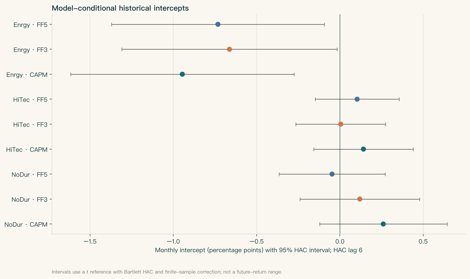
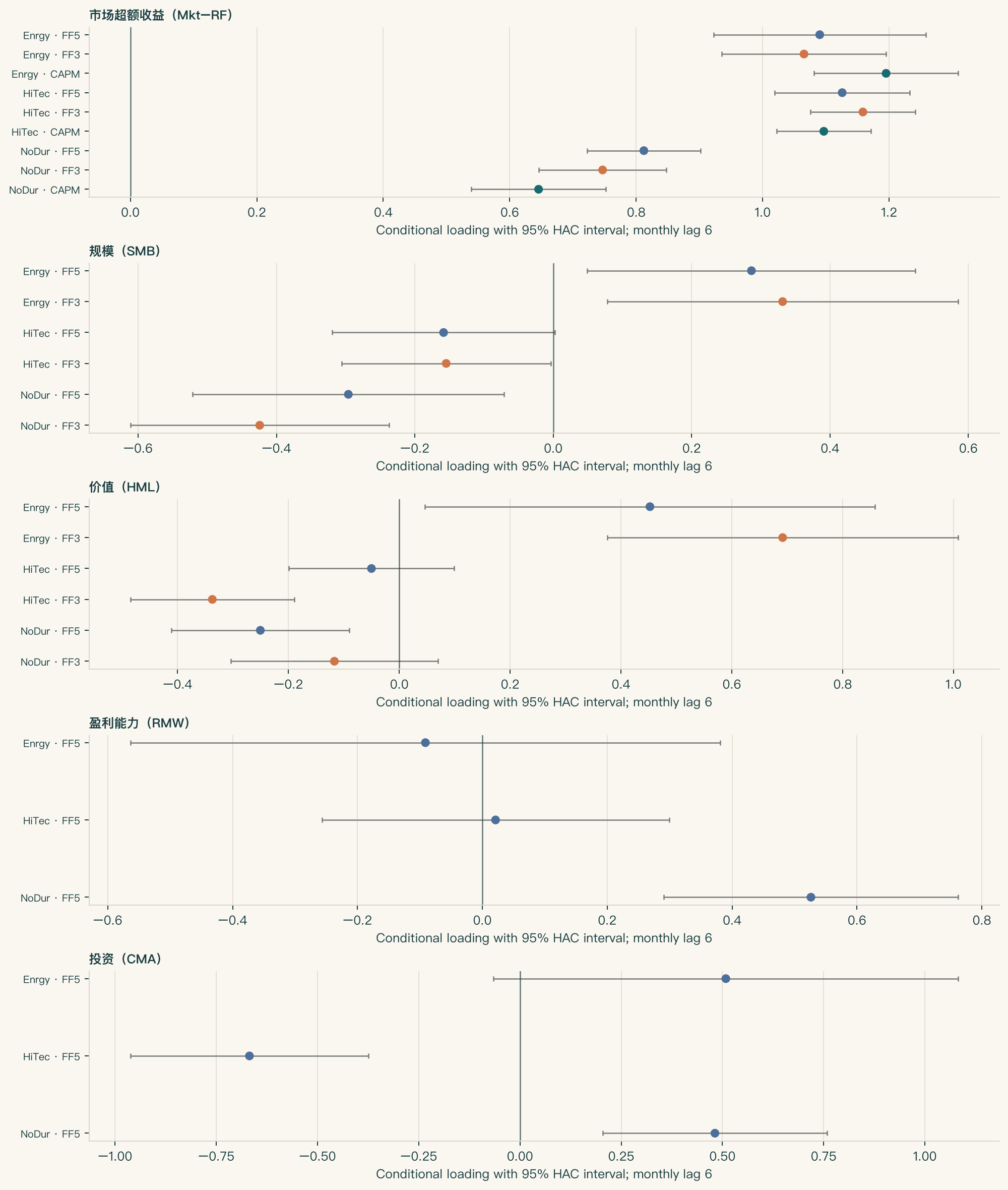
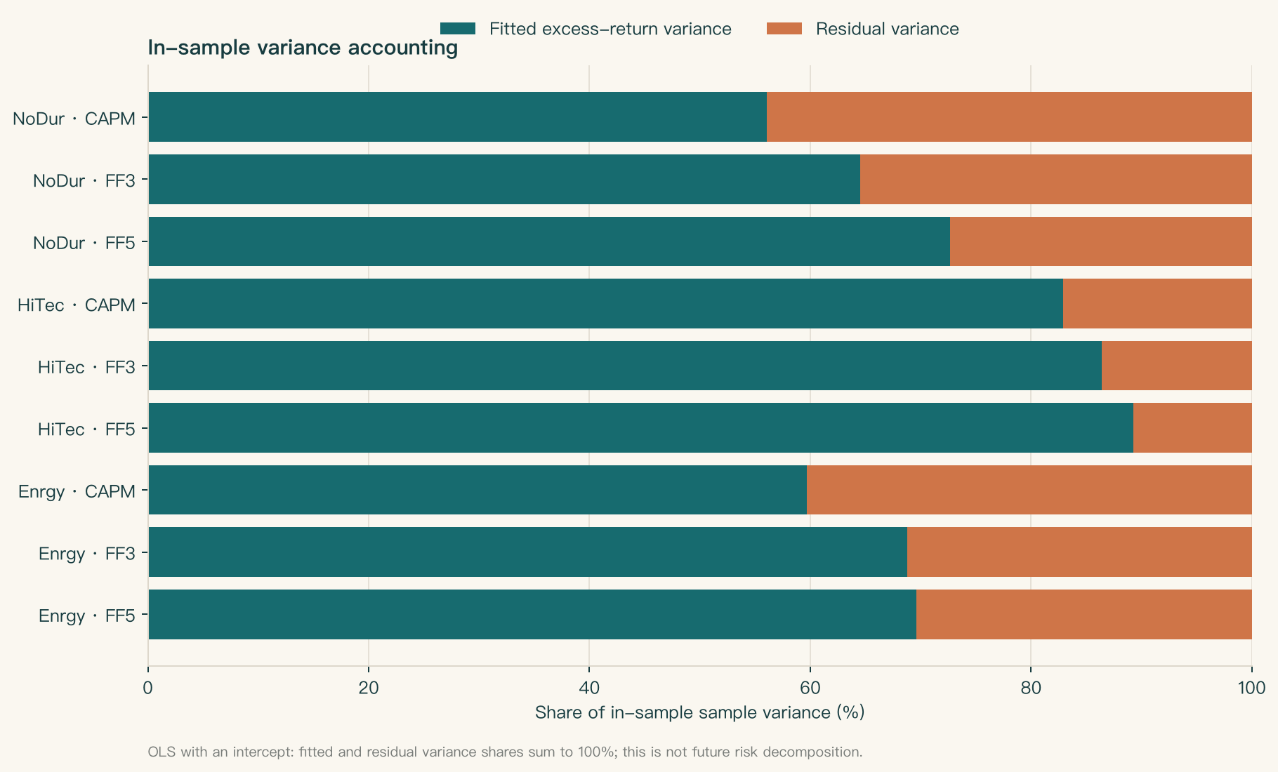
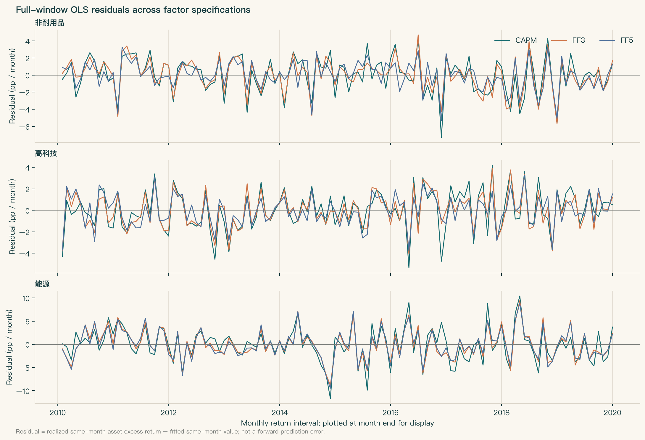
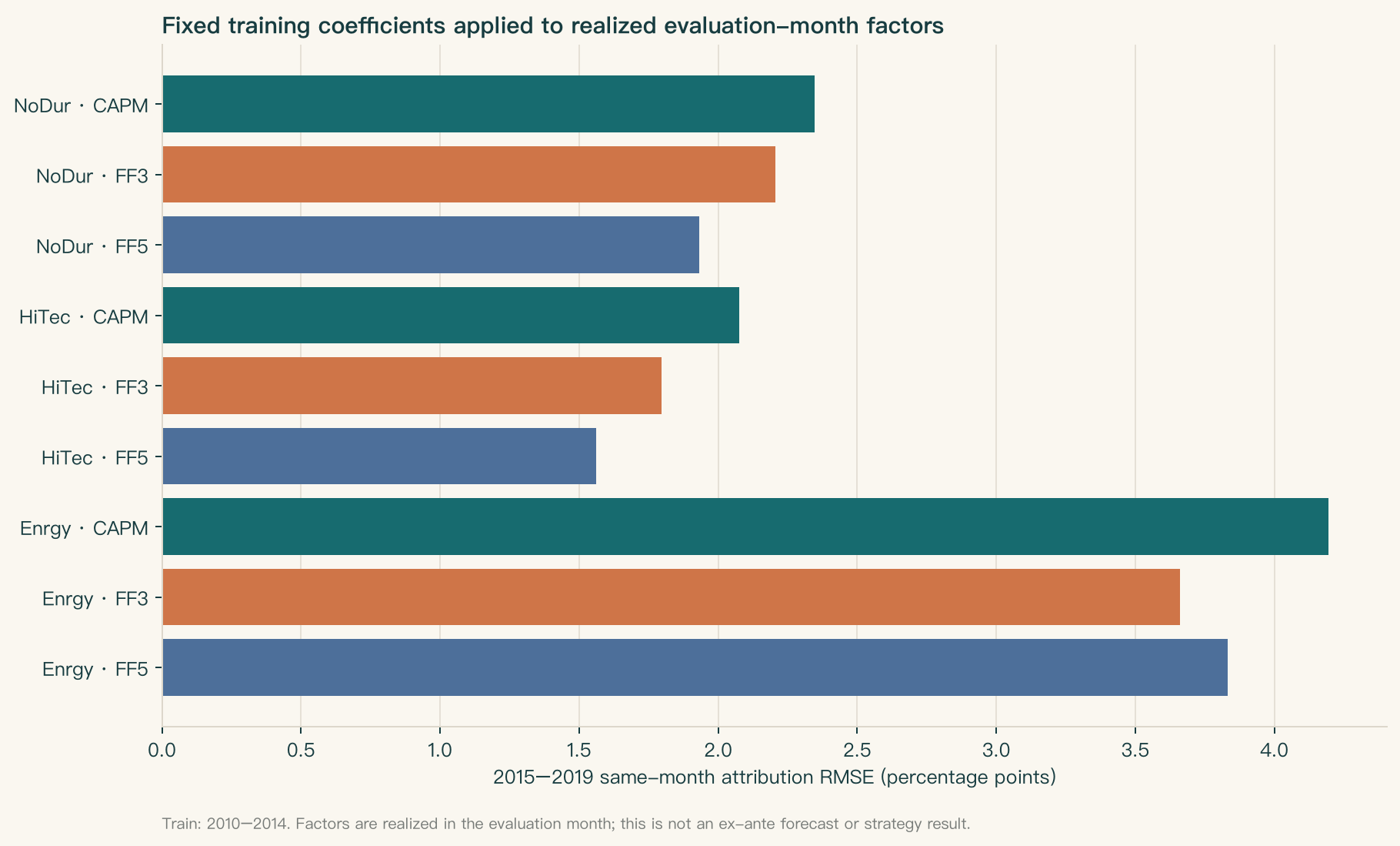
These figures summarize the original historical analysis. The common Mkt-RF and SMB series in the historical official FF3 and FF5 files differ, so those models are not strictly nested. The current constructed notebook uses the same factor columns in all three specifications. Do not compare fit or Alpha across these evidence tracks as though they measured the same market relationship.
Reading the historical report and exercises
The historical report preserves the 120-month 2010–2019 French snapshot and all results from the nine historical regressions, including negative and near-zero estimates, HAC 3/6/12 intervals, nine-test Holm adjustment, sample variance accounting, and the contemporaneous attribution check from 2010–2014 training to 2015–2019. HiTec–FF5 attribution RMSE is 1.562 and NoDur–FF5 is 1.932 percentage points per month. These are same-month factor-attribution errors, not ex ante forecast errors.
The questions cover, in order: 1) RF and factor units; 2) conditional Beta; 3) model Alpha; 4) the sample variance identity; 5) comparability of historical FF3 and FF5; 6) HAC bandwidth; 7) negative results and multiple testing; and 8) information availability and data needed for net Alpha. The solutions retain the full reasoning and evidentiary limits.
Costs, financing, and borrowing are not applicable to the historical report because there is no trading signal, target position, order, execution price, or ledger; they were not set to zero. Public access to French downloads does not grant redistribution rights. The reader package contains no raw, extracted, or processed data; G01 rights, subject, and use remain unknown, and G05 does not authorize A10-B. The default constructed demonstration does not change these gates or test market results.
The retained loading-figure Chinese panel titles mean market excess return (Mkt-RF), size (SMB), value (HML), profitability (RMW), and investment (CMA), from top to bottom. The residual-figure panel titles mean nondurables (NoDur), high technology (HiTec), and energy (Enrgy), from top to bottom. The three model colors are teal CAPM, orange FF3, and blue FF5. English bitmap titles remain a BIL23 assembly task; these historical image bytes are retained.