Risk Management

Main thread: Turn portfolio positions into a loss distribution with an explicit direction, unit, horizon, and set of conditions. Identify which exposures generate losses, which scenarios amplify them, and how the risk constraint feeds into the next executable target weights. Prerequisites: Chapter 15 on factor models, Chapter 18 on volatility, Chapter 21 on portfolio exposures, Chapter 29 on the ledger, Chapter 30 on bias, Chapter 31 on validation, and Chapter 32 on inference. After this chapter, you should be able to define VaR and ES, recompute a discrete tail, distinguish sources of risk, revalue actual ledger positions, set liquidity and margin constraints, and correctly interpret a VaR backtest.

1. Learning Objectives

After completing this chapter, you should be able to start from explicit positions and a return frequency, define the loss variable, and consistently state both the confidence level and holding horizon. You should be able to define Value-at-Risk (VaR) as a quantile and Expected Shortfall (ES) by quantile integration and threshold-atom probability; explain when ES differs from a strict-tail or inclusive-threshold conditional mean; compare historical, normal, Student-t, and Monte Carlo estimates on the same portfolio; report net exposure, gross exposure, leverage, concentration, factor exposure, liquidation days, and margin separately; apply scenario shocks to the actual positions in Chapter 29; calculate VaR exceedances using data outside the training window and explain the limits of the Kupiec unconditional coverage test; and finally convert risk limits into next-period target weights that Chapter 29 can execute.

The completion standard is not memorizing a “safe number.” You should be able to recompute outputs from inputs, identify where parameters came from, distinguish constructed scenarios from empirical data, check when information became available, and state what a metric cannot answer. Numerical examples in the body can be found in the CLI artifact ch33_results.json; each example lists its corresponding JSON keys for item-by-item reconciliation.

2. Why Quant Needs This

Chapter 29 already converts target weights into a NAV ledger with signal dates, delayed execution, fees, cash, and positions. Chapter 30 explains that an incorrect timestamp or execution assumption can inflate NAV without causing a program error. Chapter 31 requires model selection and final evaluation to be kept separate, while Chapter 32 cautions against treating a strong return curve as direct evidence of future performance. This chapter carries those lessons forward to a more specific question: how much could the positions already generated lose over a stated horizon? Could the loss come from direction, concentration, common factors, tails, liquidity, or financing constraints?

Researchers often reduce risk to volatility and multiply it by a rule-of-thumb factor. That can miss skewness, fat tails, jumps, concentrated positions, changing correlations, gaps, trading impact, and margin. A model's low VaR does not mean its extreme losses are mild. Nor do two portfolios with the same variance necessarily have the same ES or liquidation path. Risk management must also reach beyond the report: if a stress loss exceeds the limit, target positions should be reduced; target weights can be executed only after the signal exists and at a permitted execution time, never by writing them back to prices that have already occurred.

This chapter uses three kinds of evidence that must not be conflated. Probability distributions and parameterized models are assumptions. Simulations with fixed inputs and random seeds are reproducible teaching constructions. The frozen industry returns are an actually published historical series, but they are revised, backfilled data. None is presented as a complete answer to portfolio risk.

3. Intuition

Start with a discrete loss variable. Record gains as negative losses. Possible outcomes are losses of −10, 0, 5, and 20, with probabilities 0.50, 0.30, 0.15, and 0.05. Let the confidence level be $\alpha=0.90$. The cumulative distribution reaches 0.50, 0.80, 0.95, and 1.00 at these outcomes, respectively, so the first loss at which cumulative probability reaches $\alpha$ is 5. Under the lower empirical definition, this is VaR.

ES asks a harder question: what is the average loss over the worst tail interval? The tail probability is $1-\alpha=0.10$. The threshold 5 accounts for probability mass 0.15, but the worst tail needs only 0.05 of it. The threshold 20 contributes another 0.05. The weighted tail average is $(5\times0.05+20\times0.05)/0.10=12.5$. The conditional mean strictly above VaR is only 20; the conditional mean at or above VaR includes all probability mass at 5 and gives 8.75. Neither is the required mean over the worst 10% tail.

This example introduces the chapter's central idea: VaR is a quantile, while ES averages over an interval of quantiles. When a distribution has an atom at the threshold, only the portion of threshold mass needed to fill the tail belongs in the calculation. The CLI expands this input into 20 equally weighted observations and saves the CDF value, VaR, ES, strict-threshold mean, and inclusive-threshold mean. See the full quantile step function and tail area in ch33_discrete_quantile_es.png.

JSON comparison: pinned_discrete_case.loss_values, probabilities, alpha, scenario_count, cdf_at_var, var, es, strict_tail_conditional_mean, and inclusive_tail_conditional_mean.

4. Mathematical Foundations

Let $V_t$ denote portfolio value at time $t$, and let $h$ denote the holding horizon. Define monetary loss as

Thus $L>0$ means a loss and $L<0$ means a gain. If using simple returns rather than monetary amounts, write the return loss explicitly as $L^R_{t,h}=-R_{t,h}$, where $R_{t,h}=(V_{t+h}-V_t)/V_t$. Monetary loss is measured in the account's currency; return loss is a dimensionless proportion. Do not compare a USD amount and a decimal return in the same column.

Every calculation in this chapter must state both $\alpha$ and $h$. For example, “VaR is 0.10” is incomplete: the reader does not know whether this is 10% of NAV, USD 0.10, or a one-month or one-day loss. The CLI's constructed portfolio uses monthly simple returns to generate negative-return losses. The ledger stress example uses positions in shares, prices in USD per share, and per-asset shocks over the same stated simple-return interval; execution occurs on the next ledger date after the signal. In an application, replace these frequencies and times with the strategy's actual trading frequency.

4.1 Dimensional Ledger for Risk Inputs

With positive NAV and no external cash flows over the same valuation interval, $L_{t,h}=V_t L^R_{t,h}$. Under scaling by a fixed positive number, VaR and ES scale by $V_t$ as well. If the NAV denominator or cash-flow definition differs, rebuild the return ledger first; do not apply this conversion directly.

Let $F_L(\ell)=P(L\leq\ell)$ be the loss CDF. In a discrete distribution, probability mass can be concentrated at a single loss value. The quantile definition uses “at least reaches,” not linear interpolation. If a sample contains ties, the empirical quantile may also fall on an atom. A continuous model usually has no atom near its quantile, but that continuity assumption must not be silently carried over to a discrete ledger or a small empirical sample.

5. Formal Definitions

At confidence level $\alpha\in(0,1)$, define VaR as the lower quantile of the loss distribution:

This is a loss threshold. It does not describe how severe losses beyond the threshold are, and it does not mean that this loss “will never be exceeded.” If a day's loss exceeds VaR, that is an exceedance. When exceedance rates are used in backtesting, the theoretical probability equals $1-\alpha$ directly only for a continuous predictive distribution or when a consistent randomization rule has been specified for threshold atoms.

This chapter defines ES as the average of the quantile function over the upper-tail confidence interval:

If $v=\operatorname{VaR}_{\alpha}(L)$, the same quantity can be written as

Right-tail ES requires the positive part of $L$ to be integrable, $E[L^+]<\infty$; otherwise, the tail mean may not exist or may be infinite. A finite empirical sample has a finite empirical mean, but inferring population ES from a finite sample still depends on tail assumptions and sample size. The quantile-integral definition and threshold-atom adjustment used here are consistent with Acerbi and Tasche; the historical A6/C15 page-level reading scope and notation conversion are recorded in source_notes.md.

6. Derivation

In the discrete example, the quantile function $u\mapsto\operatorname{VaR}_u$ is a step function. Split the tail integral over intervals where the quantile is constant, then divide by the tail length $1-\alpha$ to obtain ES. For a distribution with a point mass, integrate only over the part of the threshold's quantile interval that is actually covered by the tail. No extra assumption that the threshold lies exactly on a probability-grid boundary is needed.

Now consider probability mass. The mass strictly above threshold $v$ is $1-F_L(v)$. The tail needs total mass $1-\alpha$, so some of the cumulative mass at or below the threshold does not belong to that tail. The difference is $F_L(v)-\alpha$; multiplying it by $v$ supplies exactly the missing threshold contribution. Add that contribution to the total loss contribution strictly above the threshold and divide by the tail probability to obtain the formula in the previous section. For a continuous distribution, $P(L=v)=0$, and at an ideal threshold $F_L(v)=\alpha$, so the adjustment vanishes. For a discrete distribution, the adjustment generally cannot be omitted.

For equally weighted observations $L_1,\ldots,L_n$, first sort $L_{(1)}\leq\cdots\leq L_{(n)}$, and let $k=\lceil n\alpha\rceil$. The empirical VaR is $L_{(k)}$. Let $v=L_{(k)}$, let $S_>$ be the sum of sample losses strictly greater than $v$, and let $m_{\leq}$ be the number of sample values at or below $v$. Then

The mathematical ceiling is defined over exact real numbers. In implementation, do not rely directly on floating-point multiplication $\texttt{alpha * n}$ followed by a ceiling: $\texttt{0.14 * 100}$ is slightly greater than 14, although empirical cumulative probability $\texttt{14 / 100}$ has already reached 0.14. The core function searches directly for the first order satisfying $\texttt{k / n >= alpha}$; regression tests also check that a probability just above 0.14 selects the next order.

This fractionally weights the sample mass at the threshold. Before computing, validate that the input is a nonempty finite real vector and that $\alpha$ lies strictly between 0 and 1; otherwise, sorting, proportions, or the denominator have no intended meaning. Convergence of empirical ES to population ES requires tail integrability and suitable sampling conditions; with few observations, the mean of the worst observations remains noisy. Acerbi and Tasche's Proposition 4.1 discusses the limit of averages of tail order statistics for independent and identically distributed samples. This does not eliminate finite-sample error or prove that a financial time series is i.i.d.

6.1 Tail Integrals for Continuous Models

For continuous $L=\mu+sZ$, $s>0$, let $z$ be the $\alpha$-quantile of $Z$. The tail probability is $1-\alpha$, and

The standard normal density satisfies $\phi'(x)=-x\phi(x)$, so

If $L\sim N(\mu,\sigma^2)$, and $z_\alpha=\Phi^{-1}(\alpha)$, then

If instead $T_\nu$ is a location-0, scale-1 Student-t random variable (not a unit-variance variable), with standardized density $f_\nu$ and quantile $t_{\nu,\alpha}$, then after location shift and scaling by $s$,

Write $f_\nu(x)=c_\nu(1+x^2/\nu)^{-(\nu+1)/2}$. Differentiate $g(x)=(1+x^2/\nu)^{-(\nu-1)/2}$:

When $\nu>1$, $g$ tends to zero at positive infinity, so

Substituting into the continuous tail integral gives the formula above; $\nu>1$ ensures an integrable tail mean. Only if $\sigma$ is interpreted as a standard deviation and the variance is matched do we need $\nu>2$. These are distinct conditions.

The Student-t mean and ES exist when degrees of freedom exceed 1; variance is finite only when degrees of freedom exceed 2. This chapter passes a mean and standard deviation, so the implementation requires $\nu>2$ and uses $s=\sigma\sqrt{(\nu-2)/\nu}$ to preserve the standard deviation. SciPy's loc and scale parameters describe location and scale; scale itself is not the Student-t standard deviation. Do not apply the familiar normal ES formula directly to a t distribution.

6.2 Kupiec Unconditional Coverage: From Likelihood to Test

Let $I_t=\mathbf1\{L_t>VaR_{t,\alpha}\}$. Under the null, assume these indicators are i.i.d. Bernoulli(q), where $q=1-\alpha\in(0,1)$. In $n$ periods with $x$ exceedances, the likelihood of the specified ordered sequence is $L(p)=p^x(1-p)^{n-x}$; if only the count is used, multiplying by the binomial coefficient does not change the likelihood ratio because it cancels.

For $0<x<n$, setting $\ell'(p)=x/p-(n-x)/(1-p)=0$ gives $\hat p=x/n$; the second derivative is negative, so this is the maximum. With zero or all exceedances, the maximum is at $p=0$ or $p=1$, respectively. Comparing fixed $q$ with free $p$,

Use $\lim_{u\downarrow0}u\log u=0$ to define zero-count log terms. When $x=0$, $LR=-2n\log(1-q)$; when $x=n$, $LR=-2n\log q$; both are finite. The commonly used $\chi^2_1$ survival function gives an asymptotic p-value; few exceedances or a boundary count do not guarantee exact small-sample calibration. Independence as Bernoulli, a continuous predictive distribution or atom randomization, threshold-estimation uncertainty, and overlapping holding periods are separate conditions to check. Splitting training and test windows does not itself establish independence. The 1,500-period/74-exceedance example in the body, the 1,082-period/5-exceedance French example, and the 250-period/0-exceedance Loom example are three different windows.

7. Financial Interpretation

Let $w_i$ be the risk-asset weight relative to NAV. Net exposure is $\sum_iw_i$; gross exposure is $\sum_i|w_i|$. In a simplified ledger with no other liabilities, cash weight can be written as $1-\sum_iw_i$. For monetary market values, divide the signed net amount and absolute gross amount by NAV to obtain net and gross leverage. Here the weights are already NAV-normalized, so leverage is the signed or absolute weight sum; do not divide by NAV again. A net exposure near zero means only that long and short market values offset; it does not mean there is no position risk, financing cost, or squeeze risk.

For a single market factor, portfolio beta can be written $\beta_p=\sum_iw_i\beta_i$. Multi-factor exposure is $B^\top w$, where each factor loading row is aligned with its asset. Dollar neutrality means net dollar exposure is zero; beta neutrality requires weighted beta to be zero; industry neutrality requires net weights to satisfy a constraint for each industry. These are different conditions. Concentration can be measured by HHI, the sum of squared weights normalized within total risk assets, or by the largest risk asset's share of total risk exposure. HHI describes weight dispersion only; it does not mean that assets are weakly correlated.

Leverage must also be read together with financing rules. Cash yield, borrow fees, rebates, funding rates, collateral haircuts, trading impact, and margin all change the cash path and the sustainable position size. The example ledger sets the per-period cash rate to 0. Borrow fees, rebates, and margin financing above the cash rate are not modeled. This simplification must not be read as saying that real financing costs are zero. Initial margin is the capital required to open a position; maintenance margin is the capital level that must not be breached while holding it. If the parameters are constructed, label them explicitly rather than presenting them as broker rules.

A stress scenario answers “what would the ledger show if these specified conditions occurred?” It is not “how likely is this?” For quantity $q_i$, current mark $P_i$, and simple-return shock $r_i$, per-asset PnL is $q_iP_ir_i$, and portfolio loss is the negative of total PnL. Setting multiple assets to adverse gaps constructs a common-shock scenario. Changing assumptions about scenario dependence does not turn this deterministic PnL into a probability model. Estimating a tail probability related to dependence requires a separately specified joint distribution and an assessment of estimation error.

Liquidity can first be approximated transparently as $D_i=|q_i|/(\pi_i\,ADV_i)$, where $ADV_i$ is shares traded per trading day, $\pi_i$ is the planned fraction of average daily volume, and $D_i$ is measured in trading days. This assumes that the position can be traded each day at the participation rate; it does not model queueing, price impact, halts, or endogenous volume. It is a capacity screen, not an execution guarantee.

8. Numerical Example

9. Python Implementation

Core functions are in risk.py, grouped by purpose:

• Distributions and tails: empirical_var_es, normal_var_es, student_t_var_es, simulate_student_t_losses.
• Revaluation and validation: scenario_pnl, lagged_rolling_var, kupiec_pof.
• Exit and financing: liquidation_days, margin_requirements.

The chapter CLI is ch33_risk_management.py. It reuses the Chapter 29 ledger, the existing exposure-report function, and the frozen French data reader.

Readers should start from the accepted I3 package root:

python run_notebook.py notebooks/ch33_risk_management.ipynb

In I3, analyze(include_french=False) skips French by default. The Notebook freshly calculates 3,000 constructed historical observations and 50,000 Monte Carlo losses, writes a results JSON, and generates four figures. It creates a unique runs/ch33_risk_management_<uuid>/; the I3 CLI uses its own runs/cli_ch33_<uuid>/. The runner also saves an execution copy, execution.json, and failure status under runs/execution_<stem>_<uuid>/. Therefore this Notebook must not be described as a static replay that writes no experiment files. This batch only inspected the entry points statically; it did not execute the full Notebook or CLI. The working-source code/ch33_risk_management.py still has an analyze() function with no include_french argument and always calls French, unlike the I3 wrapper; the two entry points must not be described as fully synchronized. The English Notebook, assembly, and cold start belong to BIL23. If a separate run is authorized, specify a new output directory and do not overwrite frozen QA results or figures.

Check core inputs separately by function. scenario_pnl (simple-return scenario revaluation) rejects non-positive prices and simple returns below −100%. Empirical loss vectors and unbounded Student-t parametric losses allow losses above 1; they belong to a different model domain and must not be hard-clipped. The Student-t API takes standard deviation and requires $\nu>2$. State the loss currency/proportion, shares, USD per share, ADV in shares per trading day, and holding period. Relevant test entry points are tests/test_ch33_risk.py and tests/test_ch33_workflow.py; this batch only makes local checks of the new display example and does not rerun the historical full workflow.

10. Visualization

The chapter CLI generates four figures; their filenames are listed in the results JSON at artifacts.figure_files.

Discrete Quantiles and ES Tail Area

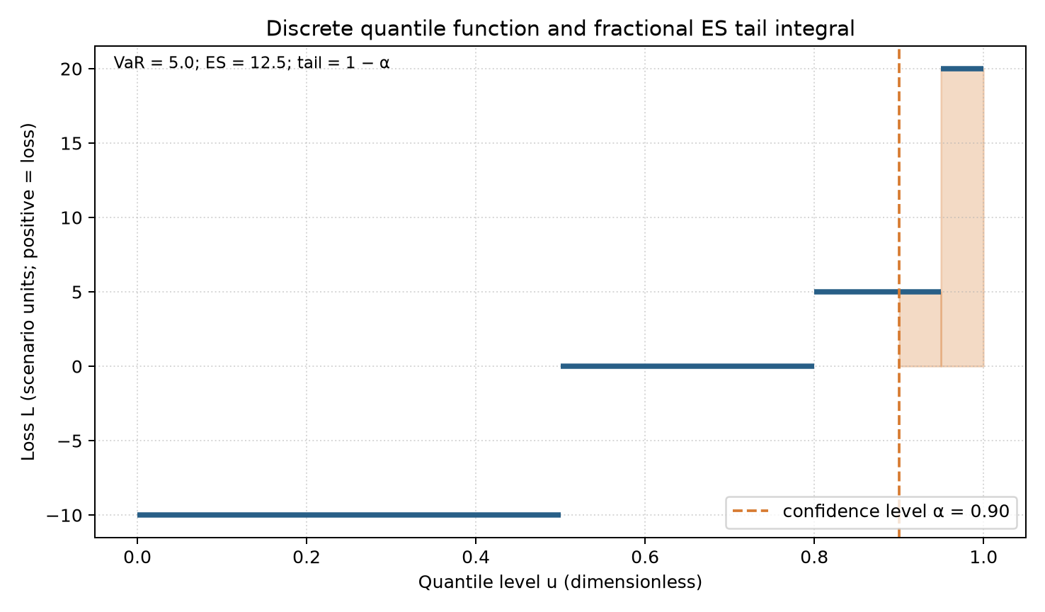
The horizontal axis is dimensionless quantile level $u$; the vertical axis is scenario loss units. The sample is the fixed discrete teaching distribution in the body. The step function is the quantile function, and the orange area includes only the quantile mass to the right of the confidence threshold. This shows why threshold value 5 contributes only the amount needed to fill the tail.

Same-Portfolio Risk Model Comparison

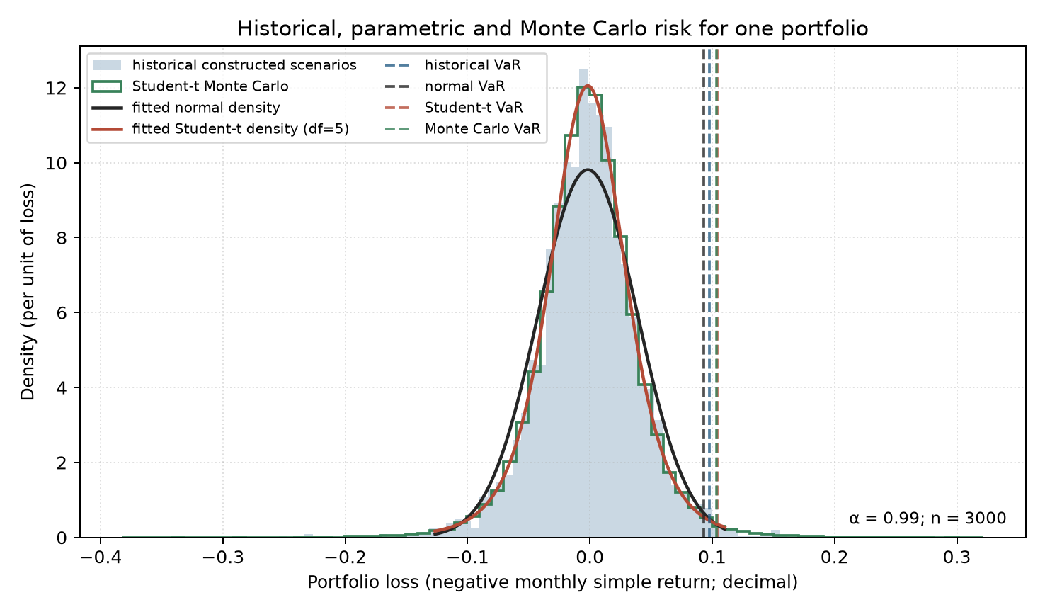
The horizontal axis is the negative of the portfolio's monthly simple return; the vertical axis is density per unit loss. The sample contains constructed historical losses and Monte Carlo losses generated from fitted Student-t parameters; the curves are normal and Student-t densities fitted to the same portfolio, and the vertical dashed lines mark the four methods' VaR. When reading the tail position, also consult the ES table. The horizontal extent of a density plot cannot establish what tails outside the model look like.

Overnight Ledger Stress Contributions

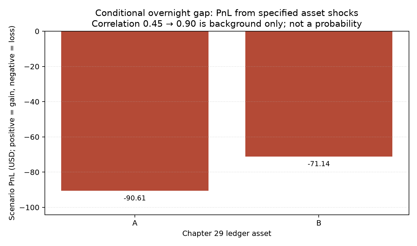
The horizontal axis lists the Chapter 29 teaching-ledger assets; the vertical axis is scenario PnL in USD, where positive is gain and negative is loss. Correlation text in the figure is a constructed state assumption, not an event probability.

Windowed VaR Backtest

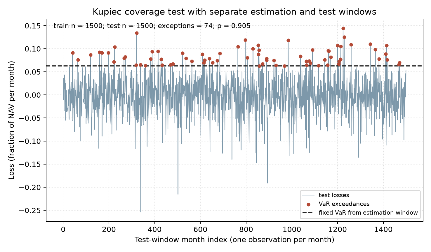
The horizontal axis is the monthly observation index within the test window; the vertical axis is NAV-proportional loss. The VaR level is estimated only from the preceding training window; red points show observations strictly above the threshold. Sample size, exceedance count, and p-value in the caption all come from the same JSON result.

A figure cannot replace explanations of parameters, sample range, fees, and timestamps. If inputs need to change, use a new output directory and rerun; do not silently overwrite existing figures or numbers.

11. Real-Market Example

In addition to constructed samples, the CLI reads the frozen Kenneth R. French Data Library monthly value-weighted returns for ten industries in the project. The input snapshot is dated 2026-10-05 and covers 1,202 months from 1926-07 through 2026-08, with ten industry portfolios. Each month, the ten published portfolios are equally weighted, using simple monthly returns. The first 120 months (1926-07 through 1936-06) form the estimation window; the remaining 1,082 months (1936-07 through 2026-08) form the test window. The training-period 95% VaR is 0.14302 and ES is 0.20204833; there are 5 exceedances in the test period, with a Kupiec LR statistic of 76.69493441 and asymptotic p-value of 1.995144691255254e−18. Reproducible fields are under JSON key french_real_example.

This is a published historical industry-portfolio series, but it is the current revised, backfilled version. It has no point-in-time version, historical receipt timestamps, or actual trades in investor-tradable constituents. The monthly label denotes the calendar period being measured, not that the return was known before month end. Nor is this a strategy trading ledger. This example can illustrate how one historical-window VaR and test-window exceedance count behave on this series; it cannot establish real-time strategy performance, trading capability, or a tradable backtest. Six SHA-256 hashes for the raw, extracted, and processed industry data and FF3 data are in french_real_example.sha256; download sources and transformation records are in data/manifests/french_industries_2026-10-05.json and the FF3 manifest. Download and use remain subject to the data provider's terms; public availability does not itself grant unrestricted redistribution rights.

12. Common Mistakes

Reversing the signs of positive return and positive loss. A positive portfolio return is a gain, but this chapter's $L=-R$ is negative. If code passes portfolio return directly to a VaR function that treats positive values as losses, the loss-tail direction is reversed. Ledger PnL uses $qPr$, and loss takes the negative; scenario_pnl returns monetary PnL, not loss.

Treating VaR as maximum loss, or writing ES as a threshold-conditional mean. VaR is not a guaranteed cap. When a distribution has probability mass at the threshold, neither the conditional mean strictly above VaR nor the conditional mean at or above VaR equals quantile-integral ES. The following code builds the same empirical sample from the results JSON and prints the correct value alongside both incorrect alternatives. Run it from the repository root:

import json
import sys
from pathlib import Path

import numpy as np

ROOT = Path.cwd()
sys.path.insert(0, str(ROOT / "src"))
from quant_course.risk import empirical_var_es

result = json.loads((ROOT / "qa/a6/codex_resume/ch33/results/ch33_results.json").read_text())
case = result["pinned_discrete_case"]
counts = np.rint(np.asarray(case["probabilities"]) * case["scenario_count"]).astype(int)
losses = np.repeat(case["loss_values"], counts)
var, es = empirical_var_es(losses, case["alpha"])
print(var, es, losses[losses > var].mean(), losses[losses >= var].mean())

The outputs are VaR, quantile-integral ES, strict-tail mean, and inclusive-threshold mean; itemized results are in pinned_discrete_case. The implementation error is usually not the sorting itself but ignoring that only part of the threshold mass belongs in the tail.

Equating high volatility with fat tails. Increasing the normal standard deviation raises tail losses but leaves the distributional shape normal. The variance-matched counterexample in the body shows that even after increasing normal VaR to the Student-t VaR, normal ES remains lower. State the distribution, parameter convention, estimation window, and frequency; “conservative volatility” alone is not enough.

Treating dollar neutrality as risklessness, or mixing gross and net into one ratio. Long and short market values can offset, while gross exposure, beta, factors, industries, borrow costs, and squeeze risk remain. A zero net position within the same industry does not mean individual securities can be liquidated easily. Report signed net and absolute gross values separately and state each denominator.

Calling scenario loss a probability, or an ADV formula an execution guarantee. A fixed return shock describes a conditional outcome. Correlation assumptions, gap size, and liquidity discounts are constructed inputs; without a calibrated model and event frequency, do not claim “the probability is X.”

Using one observation both to estimate VaR and to check its exceedance. This lets the threshold adapt to the loss already observed and creates look-ahead bias. Estimate fixed historical VaR from a training window first, then count exceedances in a later, separate test window. For rolling VaR at target period $t$, use only lookback data before $t$; the training-index interval must not contain $t$.

Treating non-rejection by the POF test as proof that the model is correct. The Kupiec test checks only whether the unconditional exceedance rate is compatible with $q=1-\alpha$; it does not determine whether exceedances cluster, tail amounts are misestimated, or predictions are stable. The degrees-of-freedom-1 chi-square p-value is asymptotic. With zero or few exceedances, the likelihood-ratio boundary can be calculated stably, but the small-sample test may have almost no power to identify a problem. Non-rejection is not proof of accuracy.

13. Quant Research Application

Place risk work in the research process by freezing the risk question first rather than choosing a statistics package. State the portfolio, currency, loss sign, confidence level $\alpha$, horizon $h$, asset set, information availability time, and decision to be supported. Fixed VaR estimates one threshold in a training window and suits a later fixed-window coverage diagnostic. Rolling historical VaR is closer to a period-by-period updated forecast, but every forecast must use only information available at that time, and calculation and backtesting must move forward by target time.

Next, check consistency between return inputs and the ledger. Availability must precede signal formation, and signal formation must precede execution. Align market prices, corporate actions, cash, fees, quantities, and return frequency. Chapter 29 target weights are not current actual weights; stress revaluation must use actual shares and marks on the correct date. If the portfolio contains options or other nonlinear positions, the linear $qPr$ shock is inadequate for repricing; use the relevant valuation model to revalue each scenario.

Then assign complementary methods to different questions: use net/gross exposure, beta, and factor exposures to locate risk sources; use VaR for a threshold at the stated confidence level; use ES for tail severity; use concentration to identify a dominant position; use ADV for a rough exit-time screen; use joint stress scenarios for conditional ledger losses; and use margin and financing assumptions to check cash constraints. Differences across methods are not a reason to pick the result that looks best; they can reveal model risk. A higher ES from a fat-tailed parametric model does not make it the true data-generating process, and a historical threshold does not automatically cover unseen events.

For model backtesting, separate the estimation and test windows. The example estimates VaR in one constructed monthly-return window and then counts strict exceedances in a non-overlapping later window. It has 74 exceedances compared with 75 expected under the null, LR statistic 0.01409458, and asymptotic p-value 0.9054967146341367. This says only that the exceedance count in this particular test window is not strong unconditional-coverage evidence against the null; it does not prove tail amounts, independence, or stability are correct. Kupiec's source notes limited power for tail validation; this chapter uses only the Bernoulli count likelihood and does not repeat the source's older wording about test properties. If clustered exceedances matter, specify a separate independence test and first read its source and finite-sample properties.

Risk limits must lead to a next-period action. In the example, the conditional-loss limit is 0.08 of current NAV; stress loss exceeds the limit, so current positions are scaled by the linear scenario-loss ratio and sent to the ledger for execution at next trading day's price. Execution has a ledger interval and includes fees and price differences; closing weights do not equal signal targets. The research report should retain the trigger value, input positions, scaling factor, filled quantities, fees, and post-trade reassessment. If costs prevent reaching the target or exit days exceed the constraint, choose a more conservative executable target rather than only changing the wording in the report.

The historical-data example uses published French industry portfolios only to demonstrate the method. The current revised industry data have no record of when they were received historically; splitting them into training and test windows cannot establish what an investor could access at the time. A real-time tradability claim requires point-in-time data, portfolio constituents, and trading-cost evidence; this example does not provide those.

13.1 Zero Exceedances: Point Probability and Test p-Value Are Different

33-L04 separately considers a 99% one-day VaR and 250 days of forecasts made in advance. Under the null of independent daily exceedances with probability 0.01, $P(X=0)=0.99^{250}\approx0.08106$ is the point probability of exactly zero exceedances. Kupiec's boundary likelihood ratio is $-500\log(0.99)\approx5.0252$; asymptotic chi-square calibration with one degree of freedom gives a p-value of about 0.025. These use different statistics or rejection regions: 8.1% is not automatically an arbitrary two-sided exact-test p-value. An exact test must first specify its one-sided or two-sided rule and discrete endpoints. The constructed backtest in the body is instead 95% monthly, with 1,500 training and 1,500 test observations; do not conflate it with this daily hand calculation.

14. Chapter Summary

A risk report should connect “what are the positions?”, “how is loss defined?”, “what information is used to estimate it?”, “how is it revalued under scenarios?”, and “how does the threshold affect the next trade?” into a traceable chain. State direction, units, confidence level, and horizon first; report VaR and ES while retaining fractional threshold mass for discrete distributions; decompose net/gross leverage, beta, factor, industry, concentration, liquidity, financing, and margin; stress actual positions rather than ideal targets; assess exceedance rates in a separate test window; and finally translate the limit into a target that can be executed after the signal at the permitted time, then reassess using actual fills.

A useful risk statement should include at least: the object and timestamp, loss sign and unit, confidence level and horizon, method and training data, VaR and ES, major factors and concentration, stress scenario and its conditional nature, liquidity and margin assumptions, out-of-sample exceedance count and test limitations, and the target and actual fills after a triggered limit. Reporting only one VaR number or one historical-backtest p-value is not enough to describe the losses a strategy can withstand.

15. Exercises

33-E01 (Discrete Threshold). Use JSON's pinned_discrete_case. Write the cumulative distribution at the loss value containing VaR, calculate the two tail contributions to ES by hand, and explain why neither the strict-exceedance mean nor inclusive-threshold mean is ES.

33-E02 (Distributional Shape). Use same_portfolio_risk_methods.variance_matched_tail_counterexample. State what is held fixed and what changes in the normal versus Student-t comparison. Explain why increasing normal standard deviation can match VaR but still fail to match ES.

33-E03 (Exposure). Use exposures. Explain the meanings of net leverage, gross leverage, cash weight, Market factor exposure, Value factor exposure, and HHI. Then use neutrality_counterexample to distinguish dollar neutrality from beta neutrality and industry neutrality.

33-E04 (Stress and Exit). Use ledger_stress_and_limit. Recompute both assets' scenario PnL from shares and prices; compare exit days under normal and stressed ADV; and explain why positive margin headroom can coexist with a triggered risk limit.

33-E05 (Coverage Test). Use risk_model_backtest. State the estimation and test window boundaries, repeat the test-window exceedance count, LR, and p-value, and name at least two conclusions that non-rejection cannot establish. Explain why the first rolling forecast can use only earlier observations.

16. Programming Exercises

33-P01 (Fractional-Tail Implementation). Read the discrete inputs from the results JSON, call empirical_var_es, and dynamically recompute VaR, ES, and both incorrect alternative means. Use assertions to verify the result keys. Tests for NaN and invalid confidence levels must raise input errors.

33-P02 (Exposure Reconciliation). Read teaching_inputs.ledger_stress from the CLI inputs and JSON output, call the existing exposure_report, and reconcile net exposure, gross exposure, and beta. Also verify that the dollar-neutral counterexample still has nonzero beta and gross exposure.

33-P03 (From Limit to Fill). Read the actual ledger shares, marks, stress returns, NAV, and cap for the signal date from JSON; call scenario_pnl to recompute stress loss and the scaling factor. Check the sign of the CLI execution orders and explain why target weights can differ from post-fill weights.

33-P04 (Kupiec Boundary). Read $\alpha$ and the test-window sample size from risk_model_backtest, call kupiec_pof to recompute the observed result, and recalculate the zero- and all-exceedance boundary likelihoods. All statistics should be finite; explain the continuous limit $0\log0=0$ and why the p-value is still asymptotically calibrated.

33-P05 (Leak-Free Rolling Forecast). Use the eight deterministic losses supplied in Section 18 (without calling the full CLI or analyze), then call lagged_rolling_var. Check that the first forecast receives only the immediately preceding window, that the output length is correct, and that no forecast contains its target-period loss.

17. Challenge Problems

33-C01 (Atoms and Risk Measures). For pinned_discrete_case, write the quantile step function and prove that the fractional-threshold formula equals the quantile integral. Then discuss how the ES result depends on integrability of the positive part of loss. If the data are negated and represented as profit, state which tail integral and sign must change.

33-C02 (What Unconditional Coverage Omits). Use the exceedance count and sample size in risk_model_backtest.test_window to construct two differently ordered exceedance sequences with the same sample exceedance rate but different clustering. Prove that Kupiec POF gives both the same likelihood-ratio statistic, and identify a further test question that requires reading and implementation.

33-C03 (Availability of a Real Series). Use french_real_example to draft a minimal research-reconciliation plan. Distinguish what the current data can and cannot support. List fields and execution evidence needed for a point-in-time interpretation of a historical simulation, and state criteria to continue, pause, or reject a strategy conclusion.

18. Solutions / Solution Hints

33-E01 Solution. The cumulative probabilities at losses −10, 0, 5, and 20 are 0.50, 0.80, 0.95, and 1.00, respectively, so the smallest loss reaching 0.90 is VaR = 5. The tail has mass 0.10; it takes all 0.05 mass at 20 and 0.05 of the mass at 5. Thus ES = (5 × 0.05 + 20 × 0.05) / 0.10 = 12.5. The conditional mean strictly above VaR is 20; the inclusive-threshold mean includes all 0.15 mass at 5 and is 8.75. The former has less than 10% tail mass, while the latter includes 20% mass; ES takes exactly the worst 10%, not an arbitrary one-sided conditional event. JSON check: pinned_discrete_case.

33-E02 Solution. The comparison holds the portfolio, loss mean, and standard deviation fixed, while changing the tail shape from normal to Student-t with 5 degrees of freedom. Normal VaR/ES are 0.09291625 and 0.10669587; the t model gives 0.10430684 and 0.13856101. Raising the normal standard deviation to 0.04556023 matches the t VaR; the normal ES rises only to 0.11974567 and remains below the t ES. The normal tail keeps its shape: a single scale change stretches the same distribution family and cannot reproduce the thicker tail shape. This counterexample does not prove that every sample is generated by a t distribution; the construction rule and seed are in teaching_inputs.portfolio_dgp.

33-E03 Solution. The target risk weights sum to 0.80, as do their absolute values, so net and gross leverage are both 0.80 and cash weight is 0.20. Market exposure is $0.50\times1.00+0.30\times1.20=0.86$; Value exposure is $0.50\times0.40+0.30\times(-0.20)=0.14$. HHI within risk assets is $(0.50/0.80)^2+(0.30/0.80)^2=0.53125$. NAV-normalized weights must not be confused with HHI normalized within risk assets. In the counterexample, weights sum to zero and absolute weights sum to 1, but beta is 0.60; the net industry amount is also zero if they are in the same industry. Therefore dollar neutrality does not imply beta neutrality, zero gross risk, or adequate liquidity.

33-E04 Solution. PnL is $q_iP_ir_i$. For A, $49.9201278\times12.1\times(-0.15)=-90.6050$ USD; for B, $14.97603834\times19\times(-0.25)=-71.1362$ USD. Negative PnL gives total conditional loss of USD 161.7412. The liquidation approximation is $D=|q|/(\text{participation rate}\times ADV)$; normal and stressed days are in ledger_stress_and_limit.liquidity. Lower ADV lengthens the exit time proportionally. Positive maintenance margin headroom is a local result under constructed margin ratios and stressed NAV. The risk limit separately compares conditional loss with an NAV fraction, so one metric being within its limit does not undo a breach of the other. Here maintenance margin headroom is USD 381.3898, yet the risk limit is breached.

33-E05 Solution. The training indices are [0, 1500), and test indices are [1500, 3000); they do not overlap. The test window has 74 exceedances, LR 0.01409458, and p-value 0.9054967146341367. Non-rejection does not prove that tail severity is accurate, exceedances are independent, the distribution is stable, or extreme stress is covered. For rolling target index 250, only indices 0 through 249 are available; including the target loss in its own threshold estimate uses the future outcome and leaks information. All fields are in risk_model_backtest.

33-P01 Reference Implementation (run from the repository root):

import json
import sys
from pathlib import Path

import numpy as np

ROOT = Path.cwd()
sys.path.insert(0, str(ROOT / "src"))
from quant_course.risk import empirical_var_es

result = json.loads((ROOT / "qa/a6/codex_resume/ch33/results/ch33_results.json").read_text())
case = result["pinned_discrete_case"]
counts = np.rint(np.asarray(case["probabilities"]) * case["scenario_count"]).astype(int)
losses = np.repeat(case["loss_values"], counts)
var, es = empirical_var_es(losses, case["alpha"])
assert np.isclose(var, case["var"]) and np.isclose(es, case["es"])
assert losses[losses > var].mean() == case["strict_tail_conditional_mean"]
assert losses[losses >= var].mean() == case["inclusive_tail_conditional_mean"]
for bad_values, bad_alpha in (([np.nan], case["alpha"]), (losses, np.nan), (losses, 0.0), (losses, 1.0)):
    try:
        empirical_var_es(bad_values, bad_alpha)
    except (TypeError, ValueError):
        pass
    else:
        raise AssertionError("non-finite input must be rejected")
print(var, es)

The assertions cover the threshold-atom adjustment. Tests also verify rejection of NaN and confidence-level boundaries; invalid inputs must not be converted into silent fill values.

33-P02 Reference Implementation (run from the repository root):

import importlib.util
import json
from pathlib import Path

import numpy as np

ROOT = Path.cwd()
spec = importlib.util.spec_from_file_location("ch33", ROOT / "code/ch33_risk_management.py")
ch33 = importlib.util.module_from_spec(spec)
spec.loader.exec_module(ch33)
from quant_course.portfolio_construction import exposure_report

result = json.loads((ROOT / "qa/a6/codex_resume/ch33/results/ch33_results.json").read_text())
inputs = ch33.INPUTS["ledger_stress"]
weights = np.asarray(inputs["initial_target_weights"])
report = exposure_report(weights, inputs["betas"], inputs["sectors"])
saved = result["exposures"]
assert report.net == saved["net_exposure"]
assert report.gross == saved["gross_exposure"]
assert report.beta == saved["market_beta"]
neutral = saved["neutrality_counterexample"]
nw = np.asarray(inputs["neutrality_example_weights"], dtype=float)
nb = np.asarray(inputs["neutrality_example_betas"], dtype=float)
assert np.array_equal(nw, [0.5, -0.5]) and np.array_equal(nb, [1.5, 0.3])
net, gross, beta = float(nw.sum()), float(np.abs(nw).sum()), float(nw @ nb)
assert net == 0 and gross == 1 and np.isclose(beta, 0.6)
assert np.isclose(net, neutral["net_leverage_on_nav"])
assert np.isclose(gross, neutral["gross_leverage_on_nav"])
assert np.isclose(beta, neutral["beta"])
print(saved["factor_exposures"], saved["concentration_hhi_within_gross_risk_assets"])

This reuses an existing exposure interface and adds no engine; industry, beta, and HHI still need to be interpreted separately.

33-P03 Reference Implementation (run from the repository root):

import json
import sys
from pathlib import Path

ROOT = Path.cwd()
sys.path.insert(0, str(ROOT / "src"))
from quant_course.risk import scenario_pnl

result = json.loads((ROOT / "qa/a6/codex_resume/ch33/results/ch33_results.json").read_text())
case = result["ledger_stress_and_limit"]
names = list(case["positions_at_signal_shares"])
pnl = scenario_pnl(
    [case["positions_at_signal_shares"][a] for a in names],
    [case["mark_prices_at_signal_currency_per_share"][a] for a in names],
    [case["overnight_gap_simple_returns"][a] for a in names],
)
loss = -float(pnl.sum())
risk = case["risk_limit"]
scale = risk["loss_cap_currency"] / loss
assert round(loss, 4) == case["conditional_stress_loss_currency"]
assert round(scale, 7) == risk["scale_factor"]
assert all(fill["quantity"] < 0 for fill in risk["actual_execution_fills"])
print(loss, scale, risk["target_weights_after_limit"], risk["actual_close_weights_after_execution"])

Sell quantities are negative. First compute the current stress loss from the actual shares held on the signal date, their current marks, and the specified return shocks. Divide the loss cap by that loss to obtain the scaling factor, then use it to form new target weights. The shares subsequently filled, execution prices, fees, and time interval all affect post-trade weights, which can therefore differ from the signal targets.

33-P04 Reference Implementation (run from the repository root):

import json
import sys
from pathlib import Path

ROOT = Path.cwd()
sys.path.insert(0, str(ROOT / "src"))
from quant_course.risk import kupiec_pof

result = json.loads((ROOT / "qa/a6/codex_resume/ch33/results/ch33_results.json").read_text())
backtest = result["risk_model_backtest"]
test = backtest["test_window"]
calculated = kupiec_pof(test["realized_exceedances"], test["observations"], backtest["alpha"])
for count in backtest["boundary_count_checks"].values():
    if isinstance(count, dict):
        edge = kupiec_pof(count["exceedances"], count["n_obs"], backtest["alpha"])
        assert edge["lr_uc"] == count["lr_uc"]
        assert edge["p_value"] == count["p_value"]
assert abs(calculated["lr_uc"] - test["lr_uc"]) < 1e-8
assert calculated["p_value"] == test["p_value"]
print(calculated)

For $x=0$ or $x=n$, kupiec_pof handles zero log terms using the continuous likelihood limit $0\log0=0$, avoiding the logarithm of zero. Boundary counts produce finite LR statistics, but the asymptotic chi-square p-value should not be read as an exact small-sample probability when exceedances are few. With all 1,500 observations as exceedances, the chi-square survival function returns 0.0 in double precision; this is numerical underflow, not an exact zero probability.

33-P05 Reference Implementation (local deterministic input; does not call the full analyze):

import numpy as np
from quant_course.risk import lagged_rolling_var

# Define a small constructor in place of the full 3,000-observation/MC/French research entry point.
def constructed_losses():
    return np.array([0.0, 0.2, -0.1, 0.4, 0.1, 0.3, -0.2, 0.5])

losses = constructed_losses()
window, alpha = 3, 0.75
actual = lagged_rolling_var(losses, window, alpha)
expected = []
for t in range(window, len(losses)):
    past = sorted(float(v) for v in losses[t-window:t])
    # Independent order-statistic selection; do not repeat empirical_var_es here.
    k = next(k for k in range(1, window+1) if k/window >= alpha)
    expected.append(past[k-1])
    changed = losses.copy()
    changed[t:] += 10.0
    altered = lagged_rolling_var(changed, window, alpha)
    np.testing.assert_array_equal(altered[:t-window+1], actual[:t-window+1])
np.testing.assert_allclose(actual, expected, rtol=0, atol=1e-14)
np.testing.assert_allclose(actual, [0.2, 0.4, 0.4, 0.4, 0.3], rtol=0, atol=1e-14)
assert len(actual) == len(losses)-window
assert expected[0] == max(losses[:3])
print(actual)

The returned item $j$ corresponds to target position $t=window+j$; each calculation independently uses only window $[t-window,t)$. Changing the loss at $t$ and afterward does not change forecasts through $t$. This example covers an explicitly finite window; it does not prove that arbitrary data or feature channels are leak-free. Missing calendar months still require a separate definition of the valid calendar. The original objective of a deterministic constructed input is retained here with a minimal explicit example, avoiding the full CLI that would call French and Monte Carlo research.

33-C01 Reference Argument. The empirical quantile function is constant on each probability-mass interval. The tail integral sums the rectangular areas strictly above the threshold, then adds the portion of the threshold interval to its right. Multiplying the threshold by $F(v)-\alpha$ gives exactly this second area. Dividing by the tail length gives the ES definition. Fractional threshold weight therefore follows directly from the discrete quantile integral; it is not an empirical patch. Generalizing to the population requires right-tail integrability $E[L^+]<\infty$. If profit is $X=-L$, with profit quantile function $q_X$, use

At an atom endpoint, negating a lower quantile requires a corresponding one-sided convention; they are not pointwise identical without it. The endpoint has measure zero in the integral, so it does not change the ES equality. See Acerbi and Tasche, Definition 2.6, Proposition 3.2, and Proposition 4.1 (the historical A6/C15 reading scope is in the source notes).

33-C02 Reference Argument. Construct two binary sequences with length test_window.observations from the results JSON. Both contain test_window.realized_exceedances ones; place the ones evenly across the first sequence and consecutively in the second. Their sample rates $x/n$ are identical. The Kupiec POF likelihood depends only on total count $x$ and sample size $n$, so both sequences have exactly the same LR and p-value; the test cannot distinguish clustering. An independence question requires conditional transitions or another sequence test. Before adding one, read its source for assumptions, zero-count handling, and finite-sample behavior. Non-rejection by POF is not a substitute for an independence test.

33-C03 Reference Argument. The current data support slicing, combining, and counting exceedances in the published monthly industry returns included in this snapshot. They do not support historical availability, historical constituents, execution prices, capacity, fees, tradable strategy returns, or future risk. A point-in-time review needs, at minimum, each version's publication and receipt time, values before and after revision, field definitions, publication timezone, historical industry membership and weights, signal availability time, order and fill records, and evidence on fees and market capacity. If versions cannot be traced, pause a real-time conclusion. If current revised values are backfilled into historical signals, reject any claim that this is leak-free deployment evidence. The exercise does not require a positive research result; credit should reward a clear distinction between “describing a historical series” and “tradable deployment.”

19. Further Reading

• Must Know: Carlo Acerbi and Dirk Tasche, On the Coherence of Expected Shortfall. The historical A6/C15 reading record for this chapter covers Definition 2.6, Proposition 3.2, equation (3.3), and relevant pages for Proposition 4.1. Use it to understand quantile integration and the ES definition at discrete threshold atoms; this is a local reading, not the full paper.
• Should Know: Paul H. Kupiec, Techniques for Verifying the Accuracy of Risk Measurement Models, FEDS 95-24. The historical A6/C15 reading record covers selected pages on daily monitoring, failure-count likelihood, binomial likelihood, and estimation error in historical simulation. Use it to understand the unconditional-coverage setup and limits on tail-validation power. This is a FEDS discussion paper; the reading was not the full journal article.
• Advanced (not read): Christoffersen's conditional coverage and exceedance-independence methods. Before using these tests, read the original work and state model assumptions, calibration, and boundary-count handling.
• Optional: Official SciPy v1.18.0 documentation for scipy.stats.t. Use it to check the ppf, pdf, rvs, loc, and scale API semantics; it is not the source for the ES derivation.
• Basel market-risk capital rules and regulatory backtesting guidance were not read for this chapter. The body makes no capital-compliance or regulatory-threshold claim.

20. References

• [AT2002-v5] Carlo Acerbi and Dirk Tasche, “On the Coherence of Expected Shortfall,” arXiv:cond-mat/0104295v5, 2002. https://arxiv.org/pdf/cond-mat/0104295v5. Historical A6/C15 citation scope: discrete-tail atom adjustment, quantile integration, and related definitions and arguments for tail-sample averages; local reading only. See source_notes.md for specific pages.
• [KUPIEC1995-FEDS95-24] Paul H. Kupiec, “Techniques for Verifying the Accuracy of Risk Measurement Models,” Finance and Economics Discussion Series 95-24, Federal Reserve Board, cover dated May 1995; interior title page dated April 1995. https://fraser.stlouisfed.org/files/docs/publications/bog_feds/feds_1995-024.pdf. The historical A6/C15 scope uses only the monitoring setup and count likelihood from the pages read; it does not generalize every claim in the source.
• [SCIPY-T] SciPy v1.18.0 Manual, scipy.stats.t. https://docs.scipy.org/doc/scipy/reference/generated/scipy.stats.t.html. The historical A6/C15 citation uses it only to confirm the Student-t API and location/scale parameterization.
• [FRENCH-FROZEN] Kenneth R. French Data Library, 10 Industry Portfolios, value-weighted monthly block; FF3 risk-free series. Industry data: https://mba.tuck.dartmouth.edu/pages/faculty/ken.french/ftp/10_Industry_Portfolios_CSV.zip; details: https://mba.tuck.dartmouth.edu/pages/faculty/ken.french/Data_Library/det_10_ind_port.html. See the corresponding project data-manifest JSON for the course's frozen snapshot, download date, use statement, processed fields, and checksums. These are current revised historical values.
• [A6-33-PLAN] Project-local frozen plan qa/a6/claude/plan.md and Chapter 33 contract terms in A6_CONTRACT.md. These support course interfaces, notation, and teaching scope, not external empirical evidence.

The historical A6/C15 reading scope, method use, and limitations for each formula and empirical result are consolidated in source_notes.md.