Performance Statistics & Inference

Thread: First describe the returns the account has realized. Then interpret the performance evidence in light of sample length, moment conditions, and the complete search record. Finally, use relative out-of-sample ranks to diagnose selection. Prerequisites: Chapter 7, Chapter 11, Chapter 22, Chapter 29, and Chapter 31. After this chapter, you will be able to calculate and interpret all 11 descriptive measures; conduct PSR and DSR significance tests and a CSCV probability-of-backtest-overfitting diagnosis; recognize multiple-testing traps; and produce a traceable performance-inference report containing byte hashes and a trial ledger. A hash is not an external timestamp or tamper-proof certification.

1. Learning Objectives

After completing this chapter, you should be able to:

1. Calculate descriptive statistics and distinguish their conventions. Keep simple returns separate from log returns, and arithmetic averages separate from the compound growth rate (CAGR), a geometric average. Calculate annualized volatility, per-period and annualized Sharpe ratios, the Sortino ratio, maximum drawdown (MaxDD), the Calmar ratio, hit rate, Profit Factor, tracking error, and information ratio; connect these measures to the turnover recorded in the actual ledger in Chapter 29.
2. Make statistical inferences under non-normality (PSR). Understand how higher moments—skewness $\gamma_3$ and kurtosis $\gamma_4$—inflate the estimated variance of the Sharpe ratio; use the Probabilistic Sharpe Ratio (PSR) formula and its one-sided hypothesis test; and distinguish the probability of skill from the probability of making money.
3. Account for selection bias and multiple testing (DSR). Understand how the maximum Sharpe ratio is inflated when the best result is selected from $N$ independent trials; derive the Deflated Sharpe Ratio (DSR) and its threshold $\mathrm{SR}_0$; and understand the heuristic estimate of the effective number of independent trials when trials are correlated.
4. Use Combinatorially Symmetric Cross-Validation and the Probability of Backtest Overfitting (CSCV/PBO). Understand the matrix-partition algorithm, relative rank $\bar{\omega}$, and the Logit transform $\lambda$; distinguish the diagnostic role of CSCV from that of a time-ordered deployment backtest (Walk-Forward).
5. Recognize inference failure conditions and empirical checks. Understand variance inflation due to serial dependence, heavy tails, and extreme regime changes, and apply the full inference workflow to the Kenneth French market data.

2. Why Quant Needs This

One of the most common illusions in a quantitative research lifecycle is the “strategy champion trap.” A researcher tries 200 combinations of moving-average periods, exit thresholds, or cross-sectional factor weights, then selects a “champion strategy” with an annualized Sharpe ratio of 2.5. The researcher reports to the investment committee with great excitement, claiming overwhelming statistical significance.

Yet six months after deployment, the strategy suffers a severe drawdown. Why can a perfect historical backtest fail to reproduce its performance in live trading?

Classical financial statistics textbooks often assume that asset returns are independent and identically distributed (i.i.d.) normal observations and test one prespecified strategy once. Modern quantitative research faces two unavoidable violations:

1. Hidden risk from non-normal returns. Hedge funds and quantitative strategies—especially mean-reversion, leveraged arbitrage, and short-volatility strategies—often exhibit negative skew and high excess kurtosis (heavy tails). Ignoring negative skew and heavy tails can substantially understate the estimation variance of the Sharpe ratio and greatly overstate statistical significance.
2. Selection bias from multiple hypothesis tests. Even if all 200 candidate models are generated by pure Gaussian white noise with no predictive power, the expected maximum sample Sharpe ratio is naturally greater than zero. Reporting only the winning point estimate without disclosing the trial search ledger is a classic form of data snooping.

A quantitative researcher therefore needs inferential statistics as well as descriptive return measures: use PSR to measure estimation uncertainty under stated moment conditions, DSR to raise the comparison threshold after a search, and CSCV to examine the relative out-of-sample ranks of candidates selected in sample.

3. Intuition

3.1 A Coin-Toss Stock-Picking Contest

Imagine a contest with 1,000 participants, each of whom tosses a coin 10 times. A head counts as a win and a tail as a loss.

For one fair-coin participant, the probability of getting 10 heads in a row is $p=2^{-10}$. The expected number of perfect records among 1,000 participants is $1000p=0.9765625$. This does not mean that exactly one participant will win every contest. If participants are also independent, the probability that at least one gets 10 heads is $1-(1-2^{-10})^{1000}\approx0.623576$. If that “champion” claims to have a special ability to predict the future, an investor who sees only the champion’s 10-for-10 record (the point estimate) may be impressed. An investor who sees the full list of 1,000 participants (the trial ledger) will recognize that the perfect record can arise as an extreme value from random sampling.

Searching for quantitative strategies works the same way:

• PSR intuition: If a participant earns very little on heads but loses heavily on tails (negative skew and heavy tails), the confidence band around the long-run Sharpe ratio is wide even if the win rate is respectable.
• DSR intuition: Given $N$ entrants, extreme-value theory raises the comparison threshold $\mathrm{SR}_0$ under the zero-skill hypothesis. Exceeding the threshold is statistical evidence against that hypothesis, but does not prove repeatable true alpha.
• CSCV intuition: Divide history into blocks. If the champion selected on some blocks tends to rank poorly relative to other candidates on the remaining blocks, the “optimization” may have selected a candidate that performs worse out of sample. The strict definition uses $\bar r<N/2$; CSCV also uses $\bar r\le(N+1)/2$.

4. Mathematical Setup

4.1 Notation and Assumptions

• Return intervals: Equal-length discrete periods $t=1,2,\dots,T$, with per-period simple returns $r_t\in(-1,+\infty)$ while the account is solvent. Wealth calculations also allow the boundary $r_t=-1$: without external capital, account wealth is then absorbed at zero and later multiplicative returns cannot revive it. A simple return below −100% requires a different negative-wealth model and is rejected by the current interface.

• Annualization factor: Let $A$ be the number of equally spaced periods in a year (daily $A=250$, monthly $A=12$).

• Benchmark and risk-free series: A risk-free return vector $r_{f,t}$ and benchmark portfolio return vector $r_{B,t}$, both at the same frequency and of equal length.

• Excess returns: $r_{e,t}=r_t-r_{f,t}$. Their sample mean and standard deviation at the same frequency are

  $$\hat{\mu}_e=\frac{1}{T}\sum_{t=1}^T r_{e,t},\qquad \hat{\sigma}_e=\sqrt{\frac{1}{T-1}\sum_{t=1}^T(r_{e,t}-\hat{\mu}_e)^2}.$$

• PSR moments: The PSR implementation estimates skewness and Pearson’s raw kurtosis from excess returns. psr_from_returns uses bias-corrected skewness and scipy.stats.kurtosis with fisher=False and bias=False. The normal benchmark has raw kurtosis $\gamma_4=3$, not excess kurtosis.

4.2 Inputs, Assumptions, and Interpretation

For a high-Sharpe curve, first ask what happened, then ask how much evidence it provides relative to a threshold. Convert frequencies before substituting values; do not add an annualized label after the calculation.

If $SR_{ann}=\sqrt A\,SR$, then $V[SR_{ann}]=A\,V[SR]$. For example, with an annualized Sharpe of 2.5 and 250 trading days per year, first compute the daily Sharpe $2.5/\sqrt{250}=0.158114$, then compare it with the daily threshold 0.113172; the difference at the same frequency is 0.044942. Compute the standard error from the native daily returns first. If these already computed quantities are then displayed consistently in annualized units, multiply the observed value, threshold, and standard error by $\sqrt{250}$; $z$ is unchanged. Do not leave daily $n$ and moments unchanged while substituting an annualized Sharpe into the per-period $D$ formula. Changing only the observed Sharpe creates spurious significance (32-L02).

The annualization convention follows from sums of returns: under independence, identical distribution, and finite variance, the mean of an $A$-period sum is $A\mu$, its standard deviation is $\sqrt A\,\sigma$, and their ratio is $\sqrt A\,\mu/\sigma$. Normality is not required for this scaling identity. Actual annual wealth from simple returns is $\prod_t(1+r_t)$, not $1+\sum_t r_t$, so this Sharpe annualization does not replace CAGR. Serial dependence requires adding the covariances across lags (32-L04).

5. Formal Definitions

5.1 Descriptive Measures

1. Wealth index and CAGR. Starting from initial capital $W_0>0$, the compounded wealth path is

   $$W_t=W_0\prod_{i=1}^t(1+r_i).$$

   Over a span of $Y$ years, the compound annual growth rate is

   $$\mathrm{CAGR}=\left(\frac{W_T}{W_0}\right)^{1/Y}-1.$$

   CAGR equals −100% if and only if bankruptcy occurs ($W_T=0$).

2. Maximum drawdown (MaxDD) and Calmar ratio. The historical wealth peak at time $t$ is $M_t=\max_{0\le s\le t}W_s$. The drawdown series is $D_t=(W_t-M_t)/M_t\in[-1,0]$. Maximum drawdown is its nonnegative absolute value, $\mathrm{MaxDD}=\max_t|D_t|$. The Calmar ratio is

   $$\mathrm{Calmar}=\frac{\mathrm{CAGR}}{\mathrm{MaxDD}}.$$

   If $\mathrm{MaxDD}=0$, Calmar is undefined and an error is raised.

3. Per-period and annualized Sharpe ratios. The per-period Sharpe ratio is defined at the native frequency of the return series and has no annualization factor:

   $$\hat{\mathrm{SR}}=\frac{\hat{\mu}_e}{\hat{\sigma}_e}.$$

   The conventional annualized Sharpe ratio is $\hat{\mathrm{SR}}_{\mathrm{ann}}=\sqrt A\,\hat{\mathrm{SR}}$.

4. Sortino ratio and downside deviation. Let the target return threshold be $\tau$ at the same frequency. The full-sample downside deviation includes all $n$ observations:

   $$\mathrm{DD}_\tau=\sqrt{\frac{1}{n}\sum_{t=1}^n\min(r_t-\tau,0)^2}.$$

   The per-period Sortino ratio is $(\bar r-\tau)/\mathrm{DD}_\tau$. Its annualized form conventionally multiplies by $\sqrt A$; downside deviation and the target do not automatically scale according to the independent-sum standard-deviation theorem. If downside deviation is zero, the ratio is undefined. The target must be finite.

5. Hit rate and Profit Factor.

   • Strict hit rate, excluding flat periods:

     $$\mathrm{HitRate}=\frac{\sum\mathbf{1}_{\{r_t>0\}}}{\sum\mathbf{1}_{\{r_t\ne0\}}}.$$

   • Profit Factor, the ratio of total gains to the absolute value of total losses:

     $$\mathrm{ProfitFactor}=\frac{\sum_{r_t>0}r_t}{|\sum_{r_t<0}r_t|}.$$

     This chapter gives each period equal weight. This is neither average winning return divided by average losing return nor a transaction Profit Factor calculated from actual monetary trade P&L. If there are no losses, Profit Factor is undefined. The hit-rate denominator excludes zero-return periods; it is also undefined when every period is flat.

6. Tracking error and information ratio. Active returns are $r_{a,t}=r_t-r_{B,t}$. Annualized tracking error is $\mathrm{TE}=\hat{\sigma}(r_a)\sqrt A$. The annualized information ratio is $\mathrm{IR}=(\bar r_a/\hat{\sigma}(r_a))\sqrt A$.

7. Ledger turnover. Connect this measure to the actual backtest ledger in Chapter 29. Turnover for one rebalance is total traded notional divided by pre-trade NAV:

   $$\mathrm{Turnover}_t=\frac{\mathrm{traded\_notional}_t}{\mathrm{nav\_pre\_trade}_t}.$$

5.2 Inference Measures

1. Probabilistic Sharpe Ratio (PSR). Under i.i.d. returns with a finite fourth moment, skewness and heavy tails adjust the estimated variance of the sample per-period Sharpe ratio. For a same-frequency benchmark $\mathrm{SR}^*$,

   $$\mathrm{PSR}(\mathrm{SR}^*)= \Phi\left( \frac{(\hat{\mathrm{SR}}-\mathrm{SR}^*)\sqrt{n-1}} {\sqrt{1-\hat{\gamma}_3\hat{\mathrm{SR}}+ \frac{\hat{\gamma}_4-1}{4}\hat{\mathrm{SR}}^2}} \right).$$

2. Deflated Sharpe Ratio (DSR). When the best Sharpe ratio is selected from $N$ independent trials, the expected maximum random Sharpe threshold under the zero-skill hypothesis is

   $$\mathrm{SR}_0=\sqrt{V[\{\hat{\mathrm{SR}}_n\}]} \left((1-\gamma)\Phi^{-1}\left(1-\frac{1}{N}\right) +\gamma\Phi^{-1}\left(1-\frac{1}{Ne}\right)\right),$$

   where $\gamma\approx0.5772156649$ is the Euler–Mascheroni constant. This uses an independent Gaussian Sharpe approximation and applies to integer $N\ge2$. Even at $N=2$ it is an approximation: the exact expected maximum of two standard normal variables is $1/\sqrt{\pi}\approx0.564190$, while the approximation gives 0.519755. With $N=1$ there is no search premium; the zero-mean noise threshold is 0, and one can use a single-test PSR. The current DSR API explicitly requires $N\ge2$ and does not substitute 1 into the inverse CDF. The expected maximum is a comparison threshold, not a critical value controlling the family-wise error rate of the whole search. DSR is not automatically an exact post-selection p-value. The Deflated Sharpe Ratio is

   $$\mathrm{DSR}=\mathrm{PSR}(\mathrm{SR}_0).$$

3. Combinatorially Symmetric Cross-Validation (CSCV) and PBO. Divide the synchronized $T\times N$ candidate return matrix by rows into an even number $S$ of equal-sized blocks. Choose any $S/2$ blocks for the in-sample set $J$ and use the complementary blocks as the out-of-sample set $\bar J$. There are $C(S,S/2)$ combinations.

   Select the best strategy in sample:

   $$n^*=\arg\max_n\hat{\mathrm{SR}}_{n,\mathrm{IS}}.$$

   Rank all $N$ strategies in the test set, with the best ranked $N$. The test-set relative rank and Logit of the strategy selected in sample are

   $$\bar{\omega}_c=\frac{\bar r_{n^*}}{N+1},\qquad \lambda_c=\ln\left(\frac{\bar{\omega}_c}{1-\bar{\omega}_c}\right).$$

   The current CSCV convention counts partitions whose test-set relative rank is at or below the midpoint: $\lambda\le0\iff\bar r\le(N+1)/2$. The local PBO Definition 2.2 instead uses $\bar r<N/2$. These are different thresholds and may produce different counts for even $N$ as well; the difference is not merely an equality convention at one shared threshold.

   $$\mathrm{PBO}_{\mathrm{CSCV}}= \frac{1}{C(S,S/2)}\sum_c\mathbf{1}_{\{\lambda_c\le0\}}.$$

6. Derivations

6.1 Algebra for the PSR Denominator Variance Term

Following Mertens (2002) and Bailey & López de Prado (2012a, Equation 8), the asymptotic variance expansion of the sample Sharpe ratio for non-normal i.i.d. returns is

Consider the two polynomial terms involving $\mathrm{SR}^2$:

Substituting this identity into the asymptotic variance expression gives

The expression above is the asymptotic variance coefficient before scaling by sample size; it is not the finite-sample variance itself. Equation (11) uses an $n-1$ denominator and substitutes sample moments to obtain the following standard-error estimate. This approximation does not become an exact finite-sample result merely because of the Bessel correction:

Under normality, $\gamma_3=0$ and $\gamma_4=3$, so the denominator term reduces to the classical Lo (2002) expression $\sqrt{1+\frac{1}{2}\hat{\mathrm{SR}}^2}$. Matching these two moments does not establish that returns are normally distributed. When $\hat{\mathrm{SR}}>0$, more negative skewness or larger raw kurtosis increases the variance term; the direction of the PSR change also depends on which side of the threshold the observed Sharpe lies, as discussed below.

The financial interpretation is to estimate the error in “mean divided by volatility” before comparing it with a threshold. Let

Then the estimator’s standard error is approximately $\sqrt{D/(n-1)}$; subtracting the threshold from the observed value and dividing by this standard error gives the PSR $z$-statistic. Increasing $n$ only reduces sampling error within a model whose conditions hold. It cannot make a nonexistent population fourth moment finite or make dependent observations independent.

The direction relative to the threshold also matters. For a fixed positive Sharpe, a moment change that increases $D$ moves PSR toward 0.5: if the observed Sharpe is above the threshold, $z$ falls and PSR moves down toward 0.5; if it is below, the negative $z$ rises toward zero and PSR moves up toward 0.5; if it equals the threshold, PSR remains 0.5. Thus, “heavy tails always lower PSR” is missing the condition that the observed value is above the threshold (32-E02).

6.2 Extreme-Value Approximation for the Maximum of Independent Standard Normals

Let $Z_1,Z_2,\dots,Z_N\overset{\mathrm{i.i.d.}}{\sim}\mathcal{N}(0,1)$, and let $M_N=\max(Z_1,\dots,Z_N)$. Its cumulative distribution function is $F_{M_N}(x)=[\Phi(x)]^N$ and its density is $f_{M_N}(x)=N\phi(x)[\Phi(x)]^{N-1}$.

The exact expected value can be calculated by numerical integration:

By extreme-value theory (the Fisher–Tippett–Gnedenko theorem), standardized normal maxima converge weakly to a Gumbel distribution. Bailey & López de Prado (2014) give the following large-sample analytic approximation using the Euler–Mascheroni constant $\gamma\approx0.5772$:

The CLI output expected_max_standard_normal_comparison reports:

• $N=10$: exact value $1.538753$, BLdP approximation $1.574598$, difference $+0.035846$;
• $N=50$: exact value $2.249074$, BLdP approximation $2.276303$, difference $+0.027229$;
• $N=100$: exact value $2.507594$, BLdP approximation $2.530603$, difference $+0.023009$.

The absolute error in these three examples decreases as $N$ grows. The acceptable error depends on the required precision; the approximation must not be described as an exact expectation.

7. Financial Interpretation

7.1 Why PSR Is Not the “Probability of Making Money”

Beginners sometimes misread $\mathrm{PSR}(0)=0.95$ as “there is a 95% probability that this strategy will make money in the future.” That is a serious statistical error.

Under i.i.d. returns with a finite fourth moment and an asymptotic normal approximation for the Sharpe estimator, $\mathrm{PSR}(\mathrm{SR}^*)$ is the normal tail area for a threshold comparison. For the one-sided null $H_0:\mathrm{SR}\le\mathrm{SR}^*$, at the boundary $\mathrm{SR}=\mathrm{SR}^*$, the corresponding approximate $p$-value is $1-\mathrm{PSR}$. Thus PSR can be expressed as a one-sided frequentist confidence level at a prespecified significance level. It is not a posterior probability about a fixed unknown parameter.

PSR measures statistical evidence for the estimated Sharpe relative to a specified threshold; it does not give the probability of a future profit-and-loss path. A strategy with 99% PSR and a small positive expected return can still have a per-period probability of loss close to 50%.

7.2 The Trial Ledger and “Alpha from Nothing”

In the chapter’s zero-skill simulation, $M=200$ independent noise strategies each have $T=1250$ daily return observations. For seed 20261032, the champion’s annualized Sharpe is 1.2318 and its naive one-sided $p$-value is 0.002941. Yet the annualized DSR threshold is 1.3257 (daily 0.083843) and DSR is 0.417160. These are results for that simulation and the DSR assumptions; they neither prove nor disprove alpha for any real strategy.

8. Numerical Examples

This section compares hand-calculation inputs and reproducible outputs from the CLI result qa/a6/codex_resume/ch32/results/ch32_results.json.

9. Python Implementation

The chapter’s core algorithms are stored in src/quant_course/inference.py; the full CLI tool is code/ch32_performance_statistics.py.

From the root of the accepted I3 reader package, run python run_notebook.py notebooks/ch32_performance_statistics.ipynb. The Notebook creates a unique runs/ch32_performance_statistics_<uuid>/ directory, computes a fresh champion example with one seed and 1,250 observations and 200 candidate strategies, and calculates 252 CSCV partitions; later cells mainly display results already held in the kernel. It is therefore more than a static replay, and the static chapter figures are not new outputs from that Notebook run. French data is skipped by default. The runner also writes an execution copy and execution.json to runs/execution_<stem>_<uuid>/; failed runs are retained too. The English Notebook and portable packaging/cold-start work belong to BIL23, and are not executed as part of this chapter workflow.

The working CLI still includes French data, multi-seed champion analysis, and AR research and should not be launched just to read this chapter. If separately authorized, use a new output directory and do not overwrite frozen QA results. The following is a local API demonstration.

import sys
from pathlib import Path
sys.path.insert(0, "src")

import numpy as np
from quant_course.inference import (
    probabilistic_sharpe_ratio,
    deflated_sharpe_ratio,
    pbo_cscv,
    per_period_sharpe,
)

# 1. Verify the PSR example from Bailey & López de Prado (2012a)
psr_norm = probabilistic_sharpe_ratio(0.458, 0.0, 24, skew=0.0, kurt=3.0)
psr_skew = probabilistic_sharpe_ratio(0.458, 0.0, 24, skew=-2.448, kurt=10.164)
psr_36m = probabilistic_sharpe_ratio(0.458, 0.0, 36, skew=-2.448, kurt=10.164)

assert round(psr_norm, 3) == 0.982
assert round(psr_skew, 3) == 0.913
assert round(psr_36m, 4) == 0.9535
print("PSR paper example verified.")

# 2. Verify the DSR example from Bailey & López de Prado (2014)
sr_daily = 2.5 / np.sqrt(250.0)
var_sr_daily = 0.5 / 250.0
dsr_100, sr0_100 = deflated_sharpe_ratio(sr_daily, var_sr_daily, 100, 1250, skew=-3.0, kurt=10.0)
dsr_46, sr0_46 = deflated_sharpe_ratio(sr_daily, var_sr_daily, 46, 1250, skew=-3.0, kurt=10.0)

assert round(sr0_100, 4) == 0.1132 and round(dsr_100, 4) == 0.9004
assert round(sr0_46, 4) == 0.1004 and round(dsr_46, 4) == 0.9505
print("DSR paper example verified.")

10. Visualization

This chapter carries forward four historical figures. For this batch, only the threshold label on the first figure is corrected using the existing six-partition cache; the historical analysis is not rerun. Figures are stored in figures/a6/, and each plot identifies its sample size, physical axis units, and theoretical data source.

10.1 Ranks and Logits for the Six Hand-Worked CSCV Partitions

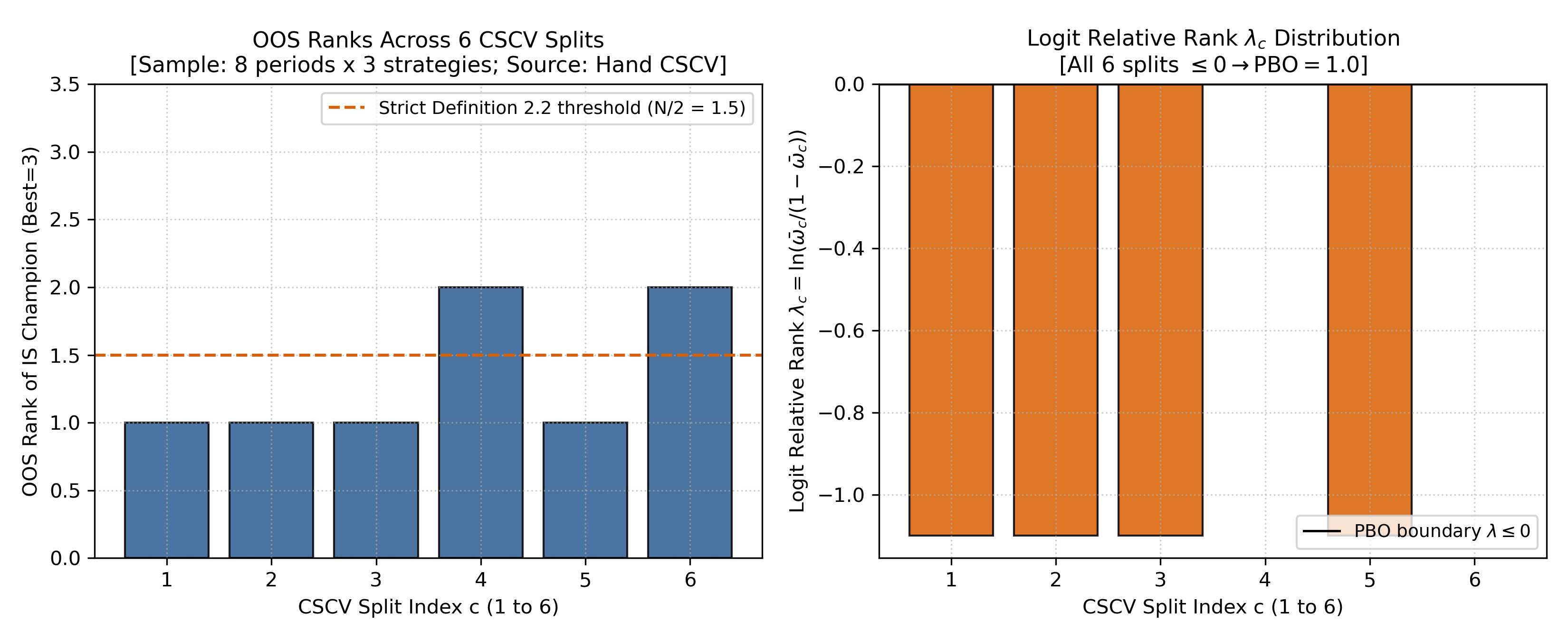
• Left plot: The horizontal axis is the index $c$ of the six combinatorial partitions; the vertical axis is the test-set rank of the in-sample winning strategy ($N=3$). The dashed line is the strict Definition 2.2 threshold $N/2=1.5$; the actual median rank of three candidates is 2.
• Right plot: The horizontal axis is the partition index and the vertical axis is the Logit statistic $\lambda_c$. All six bars are $\le0$ (partitions 4 and 6 are exactly zero), illustrating why $\mathrm{PBO}=1.0$.

10.2 Non-Normality Penalty in the Probabilistic Sharpe Ratio (PSR)

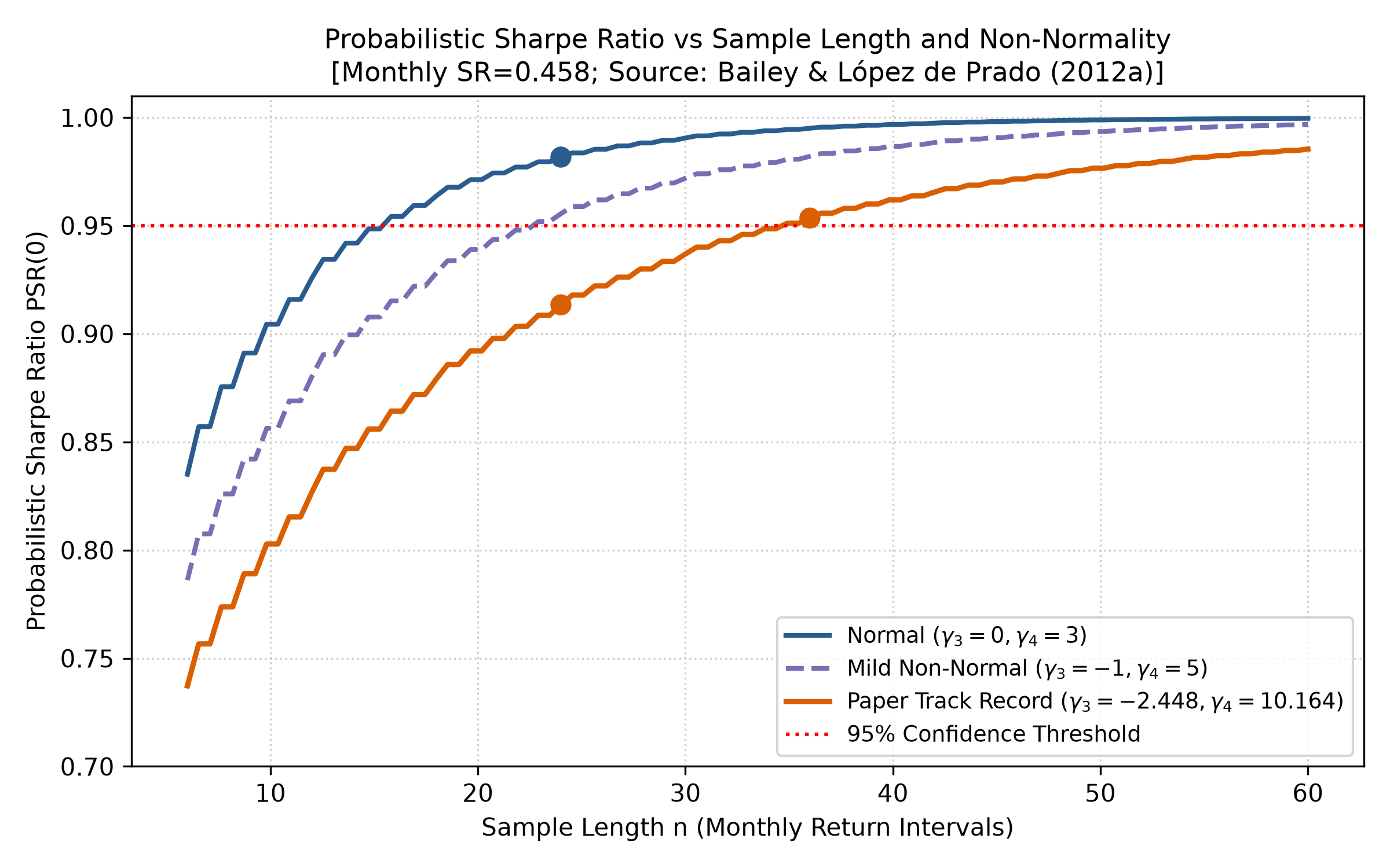
• Horizontal axis: Sample length $n$ (monthly periods, from 6 to 60 months).
• Vertical axis: $\mathrm{PSR}(0)$; the red dashed line marks a 95% confidence level.
• Observation: For these fixed inputs, normal moments give $\mathrm{PSR}(0)=0.982$, while negative-skew, heavy-tailed moments give 0.913 at $n=24$. Increasing the latter sample length to $n=36$ gives 0.9535. If a decision-maker prespecifies a one-sided 95% threshold, this 36-month example crosses it. This is a sensitivity calculation for specified moments and an observed Sharpe, not a general minimum-sample-size result.

10.3 Penalty for the Number of Trials in the Deflated Sharpe Ratio (DSR)

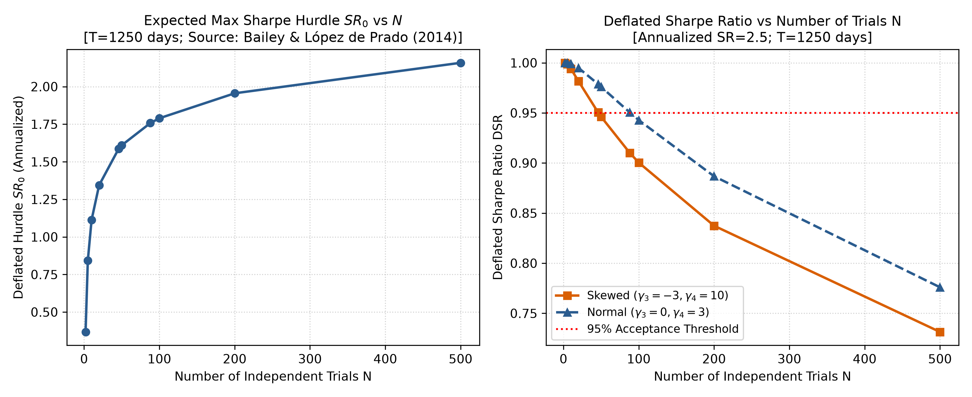
• Left plot: The horizontal axis is the number of independent trials $N$ (shown range 2–500); the vertical axis is the expected extreme-value threshold $\mathrm{SR}_0$ for annualized random Sharpe ratios.
• Right plot: The horizontal axis is the trial count $N$; the vertical axis is the DSR threshold-comparison measure under the stated assumptions.
• Observation: The figure reproduces Bailey & López de Prado (2014), Exhibit 2, over the trial-count range 2–500. At the specified points $N=46$ and $N=100$, the threshold $\mathrm{SR}_0$ rises. For an annualized Sharpe of 2.5 and the prespecified 0.95 criterion, DSR is 0.9505 at $N=46$ and 0.9004 at $N=100$. This conditional approximation does not prove true alpha or general deployment eligibility.

10.4 Comparing the Champion-Trap Experiment Distributions

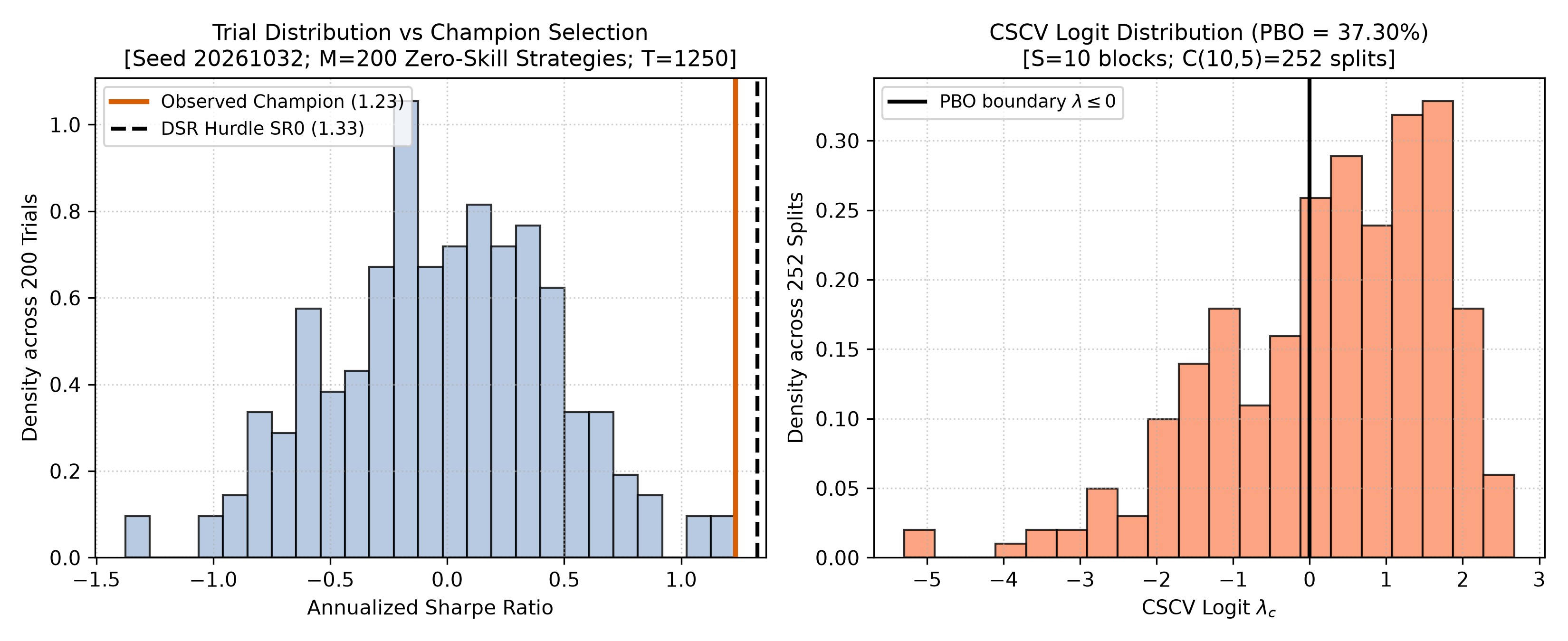
• Left plot: The Sharpe distribution of $M=200$ pure-noise candidates in one constructed world, with the selected champion marked; this is not a sampling distribution of champions across repeated worlds.
• Right plot: The distribution of CSCV Logit values $\lambda_c$, describing deterioration in the selected champion’s relative out-of-sample rank. A negative Logit does not mean an absolute loss. In the French example in Section 11, PBO is 28.14% while the fraction of out-of-sample losses is 0%, demonstrating the distinction.

11. Real-Market Example

11.1 A 100-Year History of Kenneth French’s 10 Industry Portfolios

We use quant_course.french_frozen.load_industries_and_rf to read the 10 Kenneth French value-weighted industry portfolios and the monthly FF3 risk-free rate. The data snapshot date is 2026-10-05. This is a revised historical series, not point-in-time data, and the industry portfolios are not strategies with transaction records.

To meet the CSCV divisibility requirement, the example takes the latest 1,200 months (1926-09 through 2026-08) and subtracts the monthly FF3 risk-free rate from each industry’s total return to obtain excess returns. Set $S=12$ (100 months per block), yielding all $C(12,6)=924$ partitions.

11.2 Disclosure of Empirical-Test Results

The french_market_experiment output reports:

1. Industry excess-return profile. The table gives the complete CLI result for the final 1,200 months. Annualized arithmetic excess return and volatility are computed from monthly statistics using factors of 12 and $\sqrt{12}$, respectively. Sharpe is calculated from monthly excess returns and then multiplied by $\sqrt{12}$. NoDur and Hlth have the highest annualized excess Sharpe ratios in this sample.

   Industry	Annualized excess return	Annualized volatility	Annualized Sharpe
   NoDur	8.01%	15.80%	0.5073
   Durbl	10.69%	28.59%	0.3740
   Manuf	9.01%	21.56%	0.4182
   Enrgy	9.30%	22.28%	0.4175
   HiTec	10.78%	24.79%	0.4348
   Telcm	6.58%	16.16%	0.4072
   Shops	9.20%	20.06%	0.4587
   Hlth	9.57%	19.07%	0.5020
   Utils	7.31%	18.82%	0.3882
   Other	7.82%	22.04%	0.3548

2. CSCV diagnostics.

   • $\mathrm{PBO}_{\mathrm{CSCV}}=28.14\%$ (pbo_cscv = 0.281385); under the strict-rank convention it is 23.59% (pbo_strict = 0.235931).
   • The fraction of out-of-sample losses is 0.00%; mean annualized in-sample/out-of-sample Sharpe is 0.5473/0.4508, with mean decay of 0.0964.
   • The regression slope of out-of-sample on in-sample Sharpe is −0.7975.

Limits on interpretation: These results describe only the revised historical industry portfolios under the selected CSCV partitions. They do not test a timing signal or industry momentum/quality factor, and they do not include trading, fills, fees, or investable capacity. CSCV preserves blocks but does not simulate deployment in chronological order. These statistics cannot establish future returns, tradable alpha, or suitability for launch.

12. Common Mistakes

12.1 Error 1: Annualizing Volatility with $\sqrt A$ for Serially Correlated Returns

• Example of the error and why it occurs: When the full weighted autocorrelation sum of asset returns is positive (as can occur with illiquid assets or smoothed private-equity valuations), one-period variance does not accumulate as if periods were independent. Blindly multiplying by $\sqrt A$ can materially understate true annualized portfolio volatility and inflate the annualized Sharpe ratio.
• Executable comparison:

import numpy as np

r = np.array([0.010, 0.011, 0.0105, 0.0115, 0.011, 0.012, 0.0115, 0.0125])
# Incorrect: multiply mechanically by sqrt(250)
naive_ann_vol = float(np.std(r, ddof=1) * np.sqrt(250.0))

# Example assumption: returns follow an AR(1) process with known phi=0.3
# Long-run variance inflation includes every lag rho_k = phi**k
phi = 0.3
if not -1.0 < phi < 1.0:
    raise ValueError("AR(1) coefficient must lie strictly between -1 and 1")
inflation = (1.0 + phi) / (1.0 - phi)
adjusted_ann_vol = float(naive_ann_vol * np.sqrt(inflation))
assert inflation > 0.0 and adjusted_ann_vol > naive_ann_vol

The exact finite-$A$ variance of a sum is

This counts the $A-k$ pairs at lag $k$. For an AR(1), $\rho_k=\phi^k$; only as a long-span approximation can the infinite sum $1+2\sum_{k\ge1}\phi^k=(1+\phi)/(1-\phi)$ replace it. The code above uses this long-run approximation, not the exact 250-period formula. For a general process, $\rho_1>0$ alone does not determine the sign of the full weighted sum.

• Numerical difference: With AR(1) parameter $\phi=0.3$, the long-run variance inflation factor is $(1+0.3)/(1-0.3)\approx1.857$, giving a standard-error inflation factor of 1.363. In empirical work, estimate $\phi$ on the training sample and report its uncertainty. For a general correlated series, use all relevant autocorrelation lags or a HAC variance estimate; a single sample $\rho_1$ is not an exact long-run variance correction.

12.2 Error 2: Substituting the Total Number of Strategy Columns $M$ for the Number of Independent Trials $N$ in DSR

• Example of the error and why it occurs: If 200 strategies are only small parameter variations, the number of columns may not equal the number of independent searches. Average Pearson correlation is also insufficient to determine the maximum-value distribution. It does not identify an exact “true independent trial count” or guarantee the direction of an adjustment. The following compares the numerical output of one explicitly stated heuristic.
• Executable comparison:

import math
from quant_course.inference import deflated_sharpe_ratio, implied_independent_trials

# Observed daily Sharpe 0.15, variance 0.002, total trials M=200
m_trials = 200
# Incorrect: treat 200 columns as 200 independent trials
dsr_naive, sr0_naive = deflated_sharpe_ratio(0.15, 0.002, m_trials, 1250)

# Heuristic sensitivity: interpolate N_hat using average correlation rho=0.5
n_hat = implied_independent_trials(m_trials, avg_corr=0.5)
dsr_heuristic, sr0_heuristic = deflated_sharpe_ratio(0.15, 0.002, int(round(n_hat)), 1250)

assert sr0_naive > sr0_heuristic
assert dsr_heuristic > dsr_naive

• Numerical difference: With average correlation 0.5, the heuristic gives noninteger $\hat N=0.5+0.5\times200=100.5$. The current API accepts integer $N$, so the example uses Python’s round(100.5) == 100 as an approximation. The API also clips the interpolation to $[1,M]$; a value above $M$ from negative correlation is returned as $M$. This is an implementation policy, not an extreme-value calibration theorem. The discretization does not change the fact that the formula is a heuristic or imply that its adjusted threshold establishes true alpha.

12.3 Error 3: Confusing the Arithmetic Mean with the Geometric Growth Rate

• Example of the error and why it occurs: Treating the simple arithmetic mean of period returns as compound performance ignores volatility drag.
• Executable comparison:

import numpy as np

# Two-period symmetric returns: +50% and -50%
r_seq = np.array([0.50, -0.50])
arith_mean = float(r_seq.mean())
geom_mean = float(np.sqrt(np.prod(1.0 + r_seq)) - 1.0)

assert arith_mean == 0.0
assert round(geom_mean, 6) == -0.133975

• Numerical difference: The arithmetic mean is 0.00%, but ending wealth is only 75% of initial capital (a geometric average return of −13.3975%). High volatility erodes compound growth and can hide bankruptcy risk behind an arithmetic-average illusion.

13. Quantitative Research Application

A Complete Performance-Inference Workflow: From Trial Ledger to Capital-Allocation Gate

An auditable quantitative-research workflow can be organized into four steps. Choose thresholds in advance for the decision at hand; PSR, DSR, and PBO do not have a universal launch threshold outside a model and risk preference.

[Step 1: Register the trial ledger]
  Record each parameter change and factor addition/removal in the TrialLedger (Chapter 22)
  Record total trials M, sample length T, and evaluation frequency
        ↓
[Step 2: Audit descriptive measures]
  Calculate CAGR, MaxDD, Calmar, volatility, hit rate, and Profit Factor
  Connect to the Chapter 29 ledger to audit turnover and slippage costs
        ↓
[Step 3: Account for non-normality and single-test significance (PSR)]
  Estimate sample skewness gamma3 and kurtosis gamma4
  Calculate PSR(0) at the native frequency and interpret it against a prespecified one-sided significance level
        ↓
[Step 4: Adjust for selection and multiple trials (DSR + CSCV)]
  Record dependence structure; if the effective number of trials is unknown, disclose the unknown and a sensitivity range instead of forcing an exact N_hat
  Calculate the expected maximum random-noise threshold SR0 and report DSR with its assumptions, frequency, and trial count
  Run CSCV with S blocks; report PBO, loss fraction, and partition performance, using thresholds set in advance for the decision

The transition from Chapter 32 to Chapter 33 is explicit: PSR, DSR, and PBO determine how to interpret performance evidence; the next chapter uses actual positions to calculate losses, exit capacity, and limits. Strong evidence does not replace risk constraints, and a search diagnostic does not directly generate a sell order.

14. Chapter Summary

14.1 Concept Map

                         [Return time series r_t]
                                    |
               +--------------------+--------------------+
               v                                         v
      [Descriptive statistics]                 [Inferential tests]
        (CAGR, MaxDD, Sharpe)                           |
               |                                +--------+--------+
               |                                v                 v
               |                        [Higher-moment]      [Multiple-test]
               |                         [adjustment]        [adjustment]
               |                         (skew/tails)       (trial ledger)
               |                                |                 |
               v                                v                 v
      [Point-estimate performance]       [PSR significance]   [DSR/PBO diagnosis]
               |                                |                 |
               +--------------------------------+-----------------+
                                                |
                                                v
                                [Capital allocation and
                                 anti-data-snooping decisions]

14.2 Disclosure Rules for a Rigorous Quantitative Performance Report

A performance report should disclose the information below and select inference methods appropriate to the question, sample, and model conditions. Do not show only the winning curve from a search or force an inference number when required conditions are missing:

1. Sample period and frequency: State the start and end dates, return sampling frequency, and annualization factor $A$.
2. Higher-moment characteristics: Report annualized volatility, the bias-corrected sample skewness $\hat{\gamma}_3$ actually used (bias correction does not guarantee strict unbiasedness for every distribution), and raw kurtosis $\hat{\gamma}_4$.
3. Actual search ledger: Disclose the total number of models $M$ tried during backtest selection, the parameter space, and the average correlation $\hat{\rho}$.
4. Inference measures: When the relevant moment, search, and candidate conditions are met, report $\mathrm{PSR}(0)$, threshold $\mathrm{SR}_0$, $\mathrm{DSR}$, or both CSCV PBO conventions. When they are not usable, explain the conditions and missing information.
5. Trading and capacity constraints: Use the actual Chapter 29 ledger to disclose average per-period turnover and estimated market-impact costs.

15. Exercises

• 32-E01 (Conceptual distinction): What time-series assumptions underlie the square-root scaling $\hat{\mathrm{SR}}_{\mathrm{ann}}=\sqrt A\,\hat{\mathrm{SR}}$? Distinguish the roles of i.i.d. returns and normality in this scaling relationship and in classical significance inference. If returns have positive first-order autocorrelation $\rho_1>0$, what bias results from applying this formula directly?
• 32-E02 (Mathematical property): In the PSR in Equation (11), assume the observed per-period Sharpe $\hat{\mathrm{SR}}>0$ is fixed. Using derivatives, analyze how the denominator variance term and PSR change when skewness $\hat{\gamma}_3$ decreases (becomes more negative) or kurtosis $\hat{\gamma}_4$ increases (heavier tails).
• 32-E03 (Extreme-value statistics): Under an independent Gaussian approximation for sample Sharpe ratios, explain why, even when the true expected return is zero, the expected maximum sample Sharpe tends to infinity as the number of trials $N\to\infty$.
• 32-E04 (Algorithm conventions): In CSCV, suppose there are an odd number of strategies, $N=3$, and the best strategy has test-set rank 2. State the difference in the conclusion from the strict rank rule in Definition 2.2 of Bailey et al. and the continuous integral estimate in Algorithm 2.3.

16. Programming Exercises

• 32-P01 (Sortino and downside deviation): Write an independent Python function to calculate the Sortino ratio, taking a return series that includes a zero return and a target threshold $\tau$. Verify the full-sample denominator convention using $n$ observations, and raise a controlled ValueError when downside deviation is zero.
• 32-P02 (DSR-threshold sensitivity): Call quant_course.inference.deflated_sharpe_ratio. For annualized variance $V=0.5$, output a table of daily and annualized expected-maximum Sharpe thresholds $\mathrm{SR}_0$ at trial counts $N\in[2,10,50,100,500]$.
• 32-P03 (Hand-reproducing CSCV for 8 observations): Use quant_course.inference.pbo_cscv on the $8\times3$ matrix in Section 8.3 and write assertions for the Logit statistic and PBO result in all six partitions.
• 32-P04 (Extracting ledger turnover): Write a test script that constructs a two-asset rotation ledger with quant_course.backtest and accurately calculates the turnover on each rebalance date with quant_course.inference.turnover_from_ledger.

17. Challenge Problems

• 32-C01 (Deriving the autocorrelation correction): Derive the asymptotic inflation factor $(1+\phi)/(1-\phi)$ for the sample-mean variance of a stationary AR(1) process $r_t=\phi r_{t-1}+\epsilon_t$, with $|\phi|<1$, relative to the i.i.d. case. Then use the CLI with a specified seed, sample length, and number of simulations to report the realized type-I error rate of a two-sided 5% normal test that ignores serial dependence, and explain the Monte Carlo sampling error.
• 32-C02 (Limits of the correlated-trial interpolation): Critique the equal-weight average-correlation interpolation $\hat N=\hat\rho+(1-\hat\rho)M$ in Appendix A.3 of the DSR. Give a counterexample showing why nonlinear dependence (such as tail dependence in a copula) can cause this linear formula to understate the true extreme-value risk.
• 32-C03 (Joint Walk-Forward and CSCV diagnostics): Design a research-review workflow that combines CSCV and a strictly forward, purged Walk-Forward procedure. Explain the question each answers and what additional trading, data, and risk evidence is still required.
• 32-C04 (Heavy tails and the PSR assumption boundary): Compare the realized one-sided 5% rejection rates for zero-mean standard normal, variance-standardized Student-$t_5$, and Student-$t_4$ returns at several values of $n$, using the sample Sharpe, skewness, and Pearson raw kurtosis in PSR. Explain why the population fourth moment of $t_4$ does not exist and therefore the finite-fourth-moment assumption for the PSR asymptotic variance formula fails. The simulation describes the behavior of this plug-in rule for the specified finite samples; it does not establish a general sample-size compensation theorem.

18. Solutions and Solution Hints

32-E01 — Suggested Answer

1. Conditions for scaling: For the sum of per-period excess returns, if the observations are i.i.d. with finite variance, then $E[\sum_{t=1}^A r_t]=A\mu$ and $\operatorname{Var}(\sum_{t=1}^A r_t)=A\sigma^2$. The Sharpe ratio of the sum is therefore $\sqrt A\,\mu/\sigma$. Normality is not required for this square-root scaling; it is an additional distributional assumption for classical normal-based confidence intervals or tests. With compounded simple returns, annual wealth is a product rather than the sum of periodic returns, so square-root annualization is usually a convention or approximation.
2. Bias from positive autocorrelation: For a stationary weakly dependent series, the variance of the sample mean scales with the long-run variance. Under an AR(1), the asymptotic factor is $1+2\sum_{k=1}^{\infty}\phi^k=(1+\phi)/(1-\phi)$. Positive first-order autocorrelation in an AR(1) makes this factor greater than 1. Using $\sqrt A$ anyway understates the standard deviation of an aggregated return and therefore overstates annualized Sharpe. For a general series, inference should use the full autocorrelation structure or a HAC standard error; $\rho_1$ alone does not determine the long-run variance.

32-E02 — Suggested Answer

The denominator variance term is

For $\hat{\mathrm{SR}}>0$:

• $\frac{\partial D}{\partial\hat{\gamma}_3}=-\hat{\mathrm{SR}}<0$. Thus, as skewness becomes more negative ( $\hat{\gamma}_3$ decreases), $D$ increases monotonically.
• $\frac{\partial D}{\partial\hat{\gamma}_4}=\hat{\mathrm{SR}}^2/4>0$. Thus, as kurtosis increases (heavier tails), $D$ increases monotonically.

The statistic is

If observed Sharpe is above the threshold, an increase in $D$ lowers $Z$ and lowers PSR under the standard normal CDF $\Phi$. If observed Sharpe is below the threshold, the negative $Z$ moves toward zero and PSR rises toward 0.5. If observed Sharpe equals the threshold, PSR is unchanged at 0.5. This calibrates estimation error in a threshold comparison.

32-E03 — Suggested Answer

By the asymptotic theory of standard normal extremes, as $N\to\infty$, the maximum of $N$ independent standard normal variables has the expansion

Since $\lim_{N\to\infty}\sqrt{2\ln N}=+\infty$, the expected maximum noise value grows without bound even when the strategy pool consists entirely of zero-mean white noise. This is a statement about an expectation under the model; it does not guarantee that every finite search produces a specified high value. Nor does the Gaussian approximation make the sample Sharpe ratio’s exact distribution Gaussian.

32-E04 — Suggested Answer

For $N=3$ and $\bar r^*=2$:

1. Definition 2.2 uses the condition $\bar r^*<N/2=1.5$. Since $2\ge1.5$, this partition is not counted as overfit.
2. Algorithm 2.3 gives relative rank $\bar\omega=2/(3+1)=0.50$ and Logit $\lambda=\ln(0.5/0.5)=0$. Its integral convention includes partitions with $\lambda\le0$, so this partition is counted as overfit.

The two rules use different thresholds: strict $r<N/2$ and CSCV $r\le(N+1)/2$. At $N=4$, the first counts only rank 1 and the second counts ranks 1 and 2. At $N=10$, they count ranks 1–4 and ranks 1–5, respectively. The difference also occurs for even $N$; choose and disclose the convention before looking at results.

32-P01 — Reference Implementation and Checks

import math
from quant_course.inference import sortino_ratio

def independent_sortino(returns, target=0.0, periods_per_year=1.0):
    x = [float(v) for v in returns]
    if not x or not all(math.isfinite(v) for v in x):
        raise ValueError("returns must be nonempty and finite")
    if not math.isfinite(target) or not math.isfinite(periods_per_year) or periods_per_year <= 0:
        raise ValueError("target and annualization must be finite; annualization positive")
    downside = math.sqrt(sum(min(v-target, 0.0)**2 for v in x) / len(x))
    if downside == 0:
        raise ValueError("downside deviation is zero")
    return (sum(x)/len(x)-target) / downside * math.sqrt(periods_per_year)

r = [0.04, 0.0, -0.02, 0.03, -0.01, 0.05, -0.03]
expected_dd = math.sqrt(0.0014 / 7)
expected = (0.06 / 7) / expected_dd * math.sqrt(12)
value = independent_sortino(r, periods_per_year=12)
assert math.isclose(value, expected, rel_tol=1e-12)
assert math.isclose(value, sortino_ratio(r, target_return=0.0, periods_per_year=12), rel_tol=1e-12)
assert not math.isclose(expected_dd, math.sqrt(0.0014 / 3))
for values, target in [([0.0, 0.02], 0.0), (r, math.nan), (r, math.inf), (r, -math.inf)]:
    try:
        independent_sortino(values, target)
    except ValueError:
        pass
    else:
        raise AssertionError("undefined/nonfinite case must fail")
print(value, expected_dd)

The zero-return observation remains in the full-sample denominator $n=7$; the denominator must not be changed to 3, the number of negative returns. For a nonzero target, subtract the same-frequency target from each observation first. Undefined cases should raise an error. The non-finite-target guard in the shared API is checked separately by a direct test of the candidate implementation.

32-P02 — Reference Implementation and Checks

import sys
from pathlib import Path
sys.path.insert(0, "src")

import math
import numpy as np
from quant_course.inference import deflated_sharpe_ratio

var_daily = 0.5 / 250.0
sr_daily = 2.5 / math.sqrt(250.0)
expected_sr0_ann = np.array([0.367523, 1.113409, 1.609589, 1.789406, 2.158463])
sr0_ann = []

for n in [2, 10, 50, 100, 500]:
    dsr, sr0 = deflated_sharpe_ratio(sr_daily, var_daily, n, 1250, skew=-3.0, kurt=10.0)
    sr0_ann.append(sr0 * math.sqrt(250))
    print(f"N={n:3d} -> daily SR0={sr0:.4f}, annualized SR0={sr0*math.sqrt(250):.4f}, DSR={dsr:.4f}")
np.testing.assert_allclose(sr0_ann, expected_sr0_ann, rtol=0.0, atol=1e-6)
print("32-P02 tests passed.")

32-P03 — Reference Implementation and Checks

import sys
from pathlib import Path
sys.path.insert(0, "src")

import numpy as np
from quant_course.inference import pbo_cscv

rows = [
    [0.02, 0.01, -0.01],
    [0.01, 0.00, 0.02],
    [-0.01, 0.02, 0.00],
    [0.03, -0.01, 0.01],
    [0.00, 0.01, 0.02],
    [-0.02, 0.03, 0.01],
    [0.01, -0.02, 0.03],
    [0.02, 0.00, -0.01]
]
res = pbo_cscv(rows, n_blocks=4)
assert res.n_splits == 6
assert res.pbo_cscv == 1.0
assert round(res.pbo_strict, 4) == 0.6667
expected_best = [0, 1, 0, 2, 0, 2]
expected_ranks = [1.0, 1.0, 1.0, 2.0, 1.0, 2.0]
expected_omega = [0.25, 0.25, 0.25, 0.50, 0.25, 0.50]
expected_lambdas = [-1.098612, -1.098612, -1.098612, 0.0, -1.098612, 0.0]
np.testing.assert_array_equal([p.best_strategy_index for p in res.partitions], expected_best)
np.testing.assert_allclose([p.oos_rank_best for p in res.partitions], expected_ranks, rtol=0.0, atol=1e-12)
np.testing.assert_allclose([p.relative_rank_omega for p in res.partitions], expected_omega, rtol=0.0, atol=1e-12)
np.testing.assert_allclose([p.logit_lambda for p in res.partitions], expected_lambdas, rtol=0.0, atol=1e-6)
print("32-P03 tests passed.")

32-P04 — Reference Implementation and Checks

import sys
from pathlib import Path
sys.path.insert(0, "src")

import pandas as pd
from quant_course.backtest import BacktestConfig, run_backtest
from quant_course.inference import turnover_from_ledger

dates = pd.date_range("2026-01-05", periods=4, freq="B")
mark = pd.DataFrame({"A": [10.0, 11.0, 12.1, 12.0], "B": [20.0, 19.0, 19.0, 21.0]}, index=dates)
execp = pd.DataFrame({"A": [10.0, 10.0, 12.0, 12.0], "B": [20.0, 20.0, 19.5, 20.0]}, index=dates)
tw = pd.DataFrame({"A": [0.5, 0.5], "B": [0.3, 0.3]}, index=[dates[0], dates[2]])
cfg = BacktestConfig(initial_cash=1000.0, fee_rate=0.002, lag=1)

res = run_backtest(mark, tw, cfg, exec_prices=execp)
turnover = turnover_from_ledger(res.ledger)

assert turnover.iloc[0] == 0.0
assert round(turnover.iloc[1], 4) == 0.7987
assert turnover.iloc[2] == 0.0
assert round(turnover.iloc[3], 4) == 0.0728
print("32-P04 tests passed.")

P04 carries forward the accepted BIL15A ledger: closing signals on dates[0] and dates[2] execute on dates[1] and dates[3], respectively, at the specified execution prices. Turnover uses pre-trade NAV as its denominator and total buy and sell notional as its numerator; the 0.002 fee rate is applied to traded notional in the self-financing ledger. Closing weights on trade dates may differ from target weights because of prices and fees, so target-weight changes cannot replace ledger turnover.

32-C01 — Challenge Argument and Rubric

• Suggested argument: For an AR(1) process, the autocovariance function is $\gamma_k=\frac{\sigma_\epsilon^2}{1-\phi^2}\phi^{|k|}$. The variance of the full sum is

  $$\operatorname{Var}\left(\sum_{t=1}^T r_t\right) =T\gamma_0+2\sum_{k=1}^{T-1}(T-k)\gamma_k.$$

  As $T$ becomes large, the inflation in the variance of the sample mean relative to the i.i.d. case is

  $$1+2\sum_{k=1}^{\infty}\phi^k=\frac{1+\phi}{1-\phi}.$$

  At $\phi=0.5$, the factor is 3, so the standard error is $\sqrt3\approx1.732$ times the i.i.d. standard error.

  The CLI’s boundary_experiments.ar1_dependence uses seed 20261032, $T=1000$, 2,000 simulated series, a two-sided normal $z$-test, and nominal $\alpha=0.05$. At $\phi=0.5$, the test that ignores dependence has a simulated rejection rate of $487/2000=24.35\%$ (the zero-correlation baseline is $87/2000=4.35\%$). This quantifies undercoverage in this finite simulation. Using a true rejection rate near 0.2435, the binomial Monte Carlo standard error is about 0.0096. Do not treat the result from one simulation as an exact population probability.

• Rubric:

  • Show the geometric-series derivation completely (40 points).
  • Give the closed form $(1+\phi)/(1-\phi)$ and explain its meaning (30 points).
  • Interpret the numerical result through type-I-error inflation or confidence-interval undercoverage (30 points).

32-C02 — Challenge Argument and Rubric

Let $X$ take values −3, −1, 1, and 3 with probability $1/4$ each, so its mean is 0 and variance is 5. Construct three joint distributions with the same complete marginals:

1. Joint distribution with the larger maximum: First choose a mapping independently: with probability $5/8$, use the adjacent swap $g=(-1,-3,3,1)$; with probability $3/8$, use the reversal $h=-X$. Then let $Y$ be the chosen mapping applied to $X$. Its joint probability matrix (rows for $X$ and columns for $Y$, each ordered as −3, −1, 1, 3) is

   $$P_H=\frac1{32}\begin{pmatrix} 0&5&0&3\\ 5&0&3&0\\ 0&3&0&5\\ 3&0&5&0 \end{pmatrix}.$$

   Every row and column sums to $8/32=1/4$. Under the adjacent swap, $E[Xg(X)]=(3+3+3+3)/4=3$; under reversal, $E[X(-X)]=-5$. The mixture covariance is therefore $(5/8)3+(3/8)(-5)=0$, so the Pearson correlation is zero. But $E[\max(X,g(X))]=(-1-1+3+3)/4=1$, while the maximum under reversal has expectation $E|X|=2$. Therefore $E[\max(X,Y)]=5/8+6/8=11/8$.

2. Independent joint distribution: Each of the 16 cells has probability $1/16$. The maximum has probabilities $(1,3,5,7)/16$ at the four support points, so its expectation is $(-3-3+5+21)/16=5/4$; covariance is zero.

3. Joint distribution with the smaller maximum: Choose $Y=X$ or $Y=-X$ with probability $1/2$ each. Each of the four cells associated with either mapping has probability $1/8$, and the marginals remain uniform. Covariance is $(5-5)/2=0$. The maximum has expectation $\tfrac12E[X]+\tfrac12E|X|=1$.

For $M=2$ and average correlation 0, the interpolation gives $\hat N=2$ in all three cases but cannot distinguish expected maxima of $11/8$, $5/4$, and 1. The independent model understates the maximum by $1/8$ in the first example and overstates it by $1/4$ in the third. Nonlinear dependence alone does not determine the direction. This is a teaching counterexample with a finite four-point marginal; it is not an exact Gaussian DSR calibration. Pearson correlation measures linear association for any variables with finite second moments, not only elliptically distributed variables, but does not characterize the full joint tail. When $M>T$, a demeaned sample matrix has rank at most $T-1$, so its correlation matrix can be singular. PCA or mutual-information dimensions can describe dependence, but are not exact trial counts without extreme-value calibration.

Rubric: 40 points for the complete marginals, joint probabilities, and moment calculations; 40 points for the three expected maxima and direction comparisons; 20 points for explaining the marginal model and DSR applicability boundary.

32-C03 — Challenge Argument and Rubric

• Suggested argument: CSCV is a symmetric, block-based diagnostic of backtest-selection bias. It uses the relative rank of candidate strategies on test blocks to measure whether the selected candidate falls below the median. It does not simulate deployment in chronological order and therefore cannot by itself test temporal progression, regime change, or causal availability. A Purged Walk-Forward procedure designed for the research question can provide a chronological out-of-sample evaluation; the two methods answer different questions. Freeze research rules and the search ledger first, use CSCV to examine selection stability, then use rolling forward windows to examine performance out of time, applying purge/embargo according to label overlap. Neither procedure guarantees future profits, executable trading, or live-trading suitability.
• Rubric:
  • Explain the difference between CSCV’s symmetric block diagnostic and Walk-Forward’s causal forward deployment logic (50 points).
  • Construct a research and risk-review workflow that combines them (50 points).

32-C04 — Challenge Argument and Rubric

• Suggested argument and reproducible simulation: A $t_4$ distribution has finite variance but an infinite population fourth moment. Therefore, the PSR asymptotic variance formula, which assumes a finite fourth moment, has no established calibration guarantee for $t_4$. The code below uses variance-standardized returns from each degrees-of-freedom distribution under a zero-mean null, estimates sample Sharpe, skewness, and Pearson raw kurtosis, and counts each simulation with $\mathrm{PSR}(0)>0.95$ as a rejection. This experiment compares the plug-in rule in finite samples; its rejection rates are not interpreted as a valid significance level under $t_4$.

import numpy as np
from scipy import stats

rng = np.random.default_rng(20261007)
reps = 20_000
observed_counts = []
for n in [24, 60, 120, 240]:
    for label, df in [("Normal", None), ("t5", 5), ("t4", 4)]:
        x = rng.normal(size=(reps, n)) if df is None else rng.standard_t(df, size=(reps, n)) * np.sqrt((df - 2) / df)
        sr = x.mean(axis=1) / x.std(axis=1, ddof=1)
        g3 = stats.skew(x, axis=1, bias=False)
        g4 = stats.kurtosis(x, axis=1, fisher=False, bias=False)
        d = 1 - g3 * sr + (g4 - 1) * sr**2 / 4
        assert np.all(d > 0)
        psr = stats.norm.cdf(sr * np.sqrt(n - 1) / np.sqrt(d))
        rejected = int(np.count_nonzero(psr > 0.95))
        observed_counts.append(rejected)
        print(n, label, rejected, rejected / reps)
np.testing.assert_array_equal(observed_counts, [935, 1267, 1280, 968, 1116, 1191, 1002, 1109, 1158, 1024, 1039, 1096])

The results for seed 20261007 are below. Within each $n$, the code generates Normal, $t_5$, and $t_4$ samples in that order:

The population raw kurtosis of $t_5$ is 9, and its fourth moment is finite; the population raw kurtosis of $t_4$ does not exist. Sample kurtosis is always a finite number in these simulations, but that does not restore the population moment condition for $t_4$. Values near 5% and their changes with $n$ describe only this Monte Carlo configuration; they do not give a general “number of months required for calibration” threshold.

• Rubric:
  • Explain the fourth-moment boundary between $t_4$ and $t_5$ and the applicability conditions for the PSR asymptotic approximation (50 points).
  • Reproduce the rejection rates, identify Monte Carlo error, and avoid extrapolating them into a general sample-size threshold (50 points).

19. Further Reading

1. Must know
   • Bailey, D. H., Borwein, J., López de Prado, M., & Zhu, J. Q. (2015). “The Probability of Backtest Overfitting.” SSRN Working Paper. Source reading note: Sections 2.1, 2.2, 3.1, and 4 are identified as read in the source manuscript.
   • Bailey, D. H., & López de Prado, M. (2014). “The Deflated Sharpe Ratio: Correcting for Selection Bias, Backtest Overfitting and Non-Normality.” Journal of Portfolio Management, 40(5). Source reading note: The relevant portions of the local author manuscript dated 2014-07-31 are identified as read; it was not compared page by page with the final journal version.
   • Bailey, D. H., & López de Prado, M. (2012a). “The Sharpe Ratio Efficient Frontier.” Journal of Risk, 15(2). Source reading note: The relevant portions of Equations 8–11 in the local author manuscript dated 2012-07 are identified as read; it was not compared page by page with the final journal version.
2. Should know
   • Lo, A. W. (2002). “The Statistics of Sharpe Ratios.” Financial Analysts Journal, 58(4), 36–52. Source reading note: Not read; listed as a classic reference for exact Sharpe-ratio corrections under serial dependence.
   • Mertens, E. (2002). “Variance of the IID estimator in Lo (2002).” Working paper, University of Basel. Source reading note: Not read; listed for the non-normal i.i.d. return asymptotic variance expansion.
3. Advanced
   • Harvey, C. R., Liu, Y., & Zhu, H. (2016). “…and the Cross-Section of Expected Returns.” Review of Financial Studies, 29(1), 5–68. Source reading note: Not read; listed for multiple-testing and factor-discovery thresholds in cross-sectional asset pricing.
   • Harvey, C. R., & Liu, Y. (2014). “Backtesting.” Working paper, Duke University. Source reading note: Not read; listed for sequential testing and double multiple-testing control.
4. Optional
   • Opdyke, J. D. (2007). “Comparing Sharpe Ratios: So Where’s the Catch?” Journal of Risk, 9(4), 31–60. Source reading note: Not read; listed for testing under broad stationarity and ergodicity assumptions.

20. References

• [PBO] Bailey, D. H., Borwein, J., López de Prado, M., & Zhu, J. Q. (2015). “The Probability of Backtest Overfitting.” SSRN Working Paper 2326253.
• [DSR] Bailey, D. H., & López de Prado, M. (2014). “The Deflated Sharpe Ratio: Correcting for Selection Bias, Backtest Overfitting and Non-Normality.” Journal of Portfolio Management, 40(5), 94–107.
• [PSR] Bailey, D. H., & López de Prado, M. (2012a). “The Sharpe Ratio Efficient Frontier.” Journal of Risk, 15(2), 13–44.
• [KENNETH_FRENCH] French, K. R. (2026). “Data Library: 10 Industry Portfolios.” Dartmouth Tuck School of Business.