Financial Model Validation

Main thread: trace the information used by every label and feature through time. Purging removes overlapping label intervals; embargo removes specified post-test feature look-backs; a causal walk-forward protocol evaluates predictions using information available at deployment time. These controls address their declared channels and do not by themselves establish that an entire research pipeline is free of leakage. Prerequisites: Chapters 7, 16, 22, 29, and 30. You will derive half-open interval overlap, calculate removal and retention sets, diagnose row-count gaps in panels, implement purged splits and nested selection, and interpret constructed and historical industry-return comparisons.

1. Chapter Objectives

A subtle source of apparent generalization is the interaction between a forward-return label and a validation boundary. When the target is a five-day return, training features may all precede the test block while their labels still include returns realized inside it. A chronological split of feature rows alone does not resolve that problem.

After this chapter you should be able to:

1. Derive the overlap condition for $I_i=(t_i,e_i]$,

   $$\max(t_i,t_j)<\min(e_i,e_j),$$

   and explain why touching endpoints do not overlap. Calculate the purge set for horizon $h$, establish the single-asset equivalence to gap=h-1 on a regular observation calendar, and derive the residual $(h-1)(N-1)$ overlapping rows in the specified balanced panel.

2. Distinguish the economic roles and directions of purge and embargo. Purge checks label intersections on both sides of a test block; embargo checks later training features whose historical support reaches back into the test span. Distinguish offline purged K-fold stability diagnostics from deployment-time walk-forward evaluation.

3. Use src/quant_course/validation.py to construct single-asset and panel splits, rolling and expanding windows, and nested selection. Fit the scaler and each candidate model only on the current inner training fold; select hyperparameters using inner validation scores. Refit on the current outer training set after selection, and use the outer test set only for evaluation.

4. Check invalid intervals, touching endpoints, irregular calendars, multiple assets per date, and labels whose availability $a_i$ is later than settlement $e_i$. Interpret numerical differences under the actual constructed or French-industry protocol.

Completion means calculating the 15-observation example by hand and reconciling it with the code:

Then follow the default I3 reader route in §9 and complete the questions and answers. The stored five-seed and historical French results are inherited evidence. This revision does not rerun the full CLI, Notebook, runner, or historical studies. Correct splits alone do not validate every input, execution, or feature channel.

2. Why Quants Need It

Validation connects feature engineering to portfolio construction, the Chapter 29 execution ledger, and Chapter 32 performance inference:

Data/features --> Validation and information-aware splits --> Portfolio targets
  (Ch 3,23–28)                 (Ch 31)                       (Ch 20–21)
    --> Ledger reconciliation (Ch 29) --> Performance inference (Ch 32)

Under genuinely IID sampling, a declared target distribution and training size, and no continued model selection using outer results, random K-fold can estimate the predictive risk of the corresponding training procedure. That does not make it an unconditional unbiased estimate of future deployment risk. Financial data present several additional issues:

• Overlapping labels. In the additive approximation $y_t^{\mathrm{add}}=\sum_{k=1}^5r_{t+k}$, adjacent labels share four realized returns. The compounded definition appears in §4.1. Both definitions require tracking the interval $(t,t+h]$; random row allocation may place the same future realized return in both training and test labels.
• Feature look-back leakage. Moving averages, momentum, and smoothing use historical observations. When a K-fold split trains on dates after a historical test block, those later training features can reach back into that test period.
• Global preprocessing. Fitting StandardScaler or PCA before splitting exposes the training procedure to test means, variances, or other distributional information.
• Rows versus dates. TimeSeriesSplit(gap=...) removes rows. With many securities on each date, four removed rows need not cover even one complete trading date.

This chapter formalizes the timing diagnosis in Chapter 30. The resulting out-of-sample candidate sequences feed the multiple-testing methods in Chapter 32, including PBO and CSCV, subject to those methods' own assumptions.

3. Intuition

3.1 Why the Last Training Labels Already Contain Test Returns

Suppose features are formed at each daily close and predict the next five trading days. Assign observations $t=0,1,2,3,4$ to training and begin testing at $t=5$. The feature rows are chronological, but examine their labels:

• The observation at close 4 predicts the return from close 4 to close 9.
• The first test observation at close 5 predicts the return from close 5 to close 10; the next predicts close 6 to close 11.
• More precisely, the training label at 4 contains $r_5,\ldots,r_9$, while the test label at 5 contains $r_6,\ldots,r_{10}$. They share four periods, $r_6,\ldots,r_9$. At close 5, $r_5$ has already been realized, while the training label remains unsettled until 9. Calling all five returns $r_5,\ldots,r_9$ future test returns would be inaccurate.

Treat each sample as an information interval, rather than a point on a row index.

3.2 The Frozen 15-Observation Example, Step by Step

Use observation starts $t\in\{0,1,\ldots,14\}$ on a regular trading calendar and horizon $h=5$. Each feature is available at its observation close. Its label covers

with daily returns $\{r_{t_i+1},\ldots,r_{t_i+5}\}$. Choose test starts $Q=\{6,7,8\}$ and all other starts as candidate training observations:

Test start 6: (6,11] contains returns 7,8,9,10,11.
Test start 7: (7,12] contains returns 8,9,10,11,12.
Test start 8: (8,13] contains returns 9,10,11,12,13.
The test-label span runs from start 6 to latest end 13.

First inspect the candidates before the test block:

• At 0, compare $(0,5]$ with $(6,11]$: $\max(0,6)=6$ is not less than $\min(5,11)=5$. Retain 0.
• At 1, $(1,6]$ contains $r_2,\ldots,r_6$, while $(6,11]$ contains $r_7,\ldots,r_{11}$. They touch at the close-6 base price but share no return increment. The overlap test gives $6<6$, which is false. Retain 1.
• At 2, $\max(2,6)=6<\min(7,11)=7$. Return $r_7$ is shared. Remove 2.
• At 3, $6<\min(8,11)=8$. Remove 3.
• At 4, $6<\min(9,11)=9$. Remove 4.
• At 5, $6<\min(10,11)=10$. Remove 5.

Thus the pre-test removal set is $\{2,3,4,5\}$ and its survivors are $\{0,1\}$.

Next inspect the candidates after the test block, comparing with the final test label $(8,13]$:

• At 9, $(9,14]$ overlaps because $9<13$. Remove 9.
• At 10, $(10,15]$ overlaps because $10<13$. Remove 10.
• At 11, $(11,16]$ overlaps because $11<13$. Remove 11.
• At 12, $(12,17]$ overlaps because $12<13$. Remove 12.
• At 13, $(13,18]$ only touches $(8,13]$: $13<13$ is false. Retain 13 at this stage.
• At 14, $(14,19]$ does not overlap because $14<13$ is false. Retain 14 at this stage.

After purge, the retained set is $\{0,1,13,14\}$.

Finally impose the declared feature embargo. Here the feature uses three past return periods, involving four prices: at 13 it uses prices on $[10,13]$, and at 14 on $[11,14]$. This is not a moving average of only three price points. Both supports reach into the test-label span ending at 13. With $m=3$, the post-test embargo band is

Starts 13 and 14 lie inside that band and are removed. The final training set is $\{0,1\}$. Purge and embargo are explicit geometric filters with different inputs.

3.3 Reconcile the Removal and Retention Ledgers

The complete one-way filtering chain is

There are $12-8=4$ survivors after purge and $4-2=2$ after embargo. Including future starts 13 and 14 makes this an offline purged-K-fold-style diagnostic, not a deployment training set available at time 6. Label ends remain $i+5$, so the last label ends at 19. Fifteen observation starts do not mean that all label returns end at 14; an actual dataset must supply those later returns or remove unsettled labels.

Two touching cases illustrate the distinction. $(1,6]$ ends with $r_6$ while $(6,11]$ starts with $r_7$. Likewise, $(13,18]$ starts with $r_{14}$ after $(8,13]$ ends with $r_{13}$. Both 1 and 13 pass purge, but 13 fails the feature embargo. Touching answers only the label-overlap question.

If a prediction is made at time 6 and label 1 settles at $e_1=6$ but is released at $a_1=7$, availability removes it first. Settlement does not automatically make a label readable.

4. Mathematical Foundations

4.1 Observation Coordinates and Trading Calendars

Let $\mathcal{T}=\{t_0,t_1,\ldots,t_{T-1}\}$ be strictly increasing trading dates. Observation $i$ has feature cutoff $t_i$, and its features may use only information in $\mathcal{F}_{t_i}$. Its label ends at $e_i>t_i$ and has support $I_i=(t_i,e_i]$.

For a common date sequence $\tau_0<\cdots<\tau_K$, write $t_i=\tau_{p_i}$ and $e_i=\tau_{q_i}$. Defining $r_k=P_{\tau_k}/P_{\tau_{k-1}}-1$ gives the compounded simple-return label

Writing the horizon as $e_i-t_i$ is appropriate only after encoding the endpoints as common observation positions. Adding $h$ directly to irregular dates is not valid. Map asset-specific settlement dates to a common ordered coordinate first.

4.2 Interval Algebra

For nondegenerate half-open intervals $I_1=(t_1,e_1]$ and $I_2=(t_2,e_2]$,

where the intersection is empty if its lower endpoint is at least its upper endpoint. Hence

When $e_1=t_2$, both bounds are $e_1$ and $(e_1,e_1]=\emptyset$. Endpoint touching does not overlap.

5. Formal Definitions

Observation time $t_i$. The feature cutoff, normally the daily close in this chapter.

Label end time $e_i$. The end of the outcome interval. Require $e_i>t_i$; the implementation raises ValueError for $e_i\le t_i$.

Availability time $a_i$. The earliest timestamp at which the settled or released label is recorded and readable. Liquid-market closing labels may have $a_i=e_i$, while fund NAVs, international assets, and financial-statement measures can have $a_i>e_i$. A deployment training label must satisfy $a_i\le t_{\mathrm{predict}}$. The current validation.py interface accepts only $t_i,e_i$, not an independent $a_i$. The caller must filter candidates using actual availability before each fit; delayed $a_i$ cannot be replaced by $e_i$.

Candidate set $C$. Construct it for the intended evaluation. Deployment walk-forward takes past observations with labels available by prediction time. Offline purged K-fold may use future training blocks whose labels are available by the later evaluation time; it cannot claim that those blocks were available for the historical prediction. Let $Q$ be the test set, with $C\cap Q=\emptyset$.

Purging. Define the removal set and then its complement:

One overlap with any test label is sufficient for removal. No overlap, including mere touching, passes this filter. Here $R$ means removed and $S$ means survivors. The panel policy conservatively checks time globally rather than exempting overlapping labels because their asset identifiers differ.

Embargo. Inspect only post-test candidates that have already passed purge:

Here $t_{\mathrm{test,max}}=\max_{j\in Q}t_j$ and $e_{\mathrm{test,max}}=\max_{j\in Q}e_j$. The buffer $m\ge0$ has the same units as the time coordinate; trading-observation periods are not automatically calendar days. This chapter chooses a buffer covering the declared maximum feature look-back. The left endpoint is included, the right excluded, and $m=0$ removes nothing. The current API converts $t,e$ to floats. It does not parse dates, reconcile asset calendars, or enforce $a$. Encode a common ordered coordinate and express $m$ in that unit. A finite buffer covers the stated finite support; it does not eliminate the infinite memory of an untruncated EMA.

The filtering invariant is

A removed sample never reappears during embargo or later concatenation. A past-only walk-forward has no post-test candidates and thus $R_{\mathrm{embargo}}=\emptyset$. Under strict deployment conditions

we already have $e_i\le\min t_j$, excluding overlap with future test returns; an explicit interval check remains a useful implementation safeguard. Offline future-block diagnostics can still require two-sided purging. Conversely, nonoverlap does not establish availability: a touching historical label may be released late.

TimeSeriesSplit gap $g$. The number of sample rows omitted between the training block and test block, not a number of dates.

Purged walk-forward. A forward-moving design with historical training candidates and a subsequent test block; check the trailing training labels for overlap.

Purged K-fold. Split time into $K$ contiguous, unshuffled blocks. For each test block, use the other past and future blocks as candidates and apply purge and embargo.

Nested validation. The outer split evaluates out-of-sample performance. Inner splits are confined to the current outer training set and select hyperparameters or features. Fit preprocessing means and variances only on the current training fold.

6. Derivations

6.1 Proof of the Necessary and Sufficient Overlap Condition

Theorem 1. For $t_1<e_1$ and $t_2<e_2$,

Proof. Membership in the intersection requires both $t_1<x\le e_1$ and $t_2<x\le e_2$. Combining the inequalities gives

Such a real $x$ exists exactly when the lower bound is strictly less than the upper bound. If so, every point in the displayed half-open interval belongs to both intervals. If the lower bound is at least the upper bound, no point satisfies both inequalities and the intersection is empty. This proves both directions.

6.2 Purge Counts and Gap Equivalence for One Regular Asset

Assume fixed integer horizon $h\ge2$ and regular observation positions, with $e_i=t_i+h$. For a contiguous test block starting at $t_{\mathrm{test}}$ and containing $n_{\mathrm{test}}$ starts, the union of its label intervals is

For a prior candidate $t_i<t_{\mathrm{test}}$, Theorem 1 reduces overlap with the first test label to

The integer starts to remove are therefore

whose count is

This count presumes those preceding observations exist. TimeSeriesSplit uses the exclusive slice end

For one regular asset, gap=h-1 sets that end to $t_{\mathrm{test}}-h+1$ and removes exactly the same trailing observations. This equivalence relies on the stated calendar, horizon, and one-row-per-date conditions.

6.3 Why the Same Row Gap Fails in a Panel

Theorem 2. Suppose a complete balanced panel has exactly $N\ge2$ assets per date, sorted by (date, asset), fixed integer horizon $h\ge2$, a test block beginning at a complete-date boundary, and at least $h-1$ preceding consecutive dates. The test date $T_{\mathrm{test}}$ begins at row $R_{\mathrm{test}}=T_{\mathrm{test}}N$. Using the row gap $h-1$ leaves exactly

overlapping training rows.

Proof. Every asset on dates $T_{\mathrm{test}}-h+1,\ldots,T_{\mathrm{test}}-1$ overlaps the test-label span. Thus the required removal count is

The row-based algorithm instead removes only

a total of $h-1$ rows. Those rows lie within the true overlap band. They cover at most $\lfloor(h-1)/N\rfloor$ complete dates and part of one further date, so the remaining count is

For the frozen $N=3,h=5$ example, dates 2–5 contain 12 overlapping rows. A four-row gap removes all three assets on date 5 and the third asset on date 4. Eight rows remain: three on date 2, three on date 3, and two on date 4. This proves the result. Missing assets or dates, variable horizons, insufficient history, or a boundary inside a date require direct interval calculations instead of this closed form.

7. Financial Interpretation

7.1 Why Do Financial Features and Labels Have Long Memory?

In classical statistics, residuals are often assumed to be independent and identically distributed white noise. Financial asset prices, however, are jointly driven by fundamentals, macroeconomic liquidity, and strategic interactions among investors.

If compounding period-by-period simple returns is approximated by summing small returns, an $h$-period label can be written as a rolling sum, $y_t^{\mathrm{add}}=\sum_{k=1}^h r_{t+k}$. When the returns $r_t$ have equal variance and are pairwise uncorrelated, as under a homoskedastic martingale difference process, the covariance at lag $0\le\ell<h$ is:

This is an exact result for additive labels; the covariance is zero when $\ell\ge h$. It is not a general exact covariance formula for the compounded simple-return label defined in §4.1.

For the compounded simple-return label in §4.1, $Y_t=\prod_{k=1}^h(1+r_{t+k})-1$, an exact expression follows only under the additional assumption that simple returns are independent and identically distributed over time. Let $G=1+r$, $m_1=\mathbb{E}[G]$, and $m_2=\mathbb{E}[G^2]$. Then, for $0\le\ell<h$:

If $\mathbb{E}[r]=0$ and $\mathrm{Var}(r)=\sigma_r^2$, this becomes $(1+\sigma_r^2)^{h-\ell}-1$, which is approximated by $(h-\ell)\sigma_r^2$ only when the variance is small. Overlapping intervals therefore induce statistical dependence between labels, but its strength depends on the return distribution, holding period, and lag. Interval overlap alone does not imply that labels are necessarily highly correlated. The Purge logic still applies: it prevents the same realized return from entering both a training label and a test label.

The effect of label overlap on model evaluation depends on the data-generating process, model, feature structure, and test window. In this chapter's Ridge construction, the average score difference before and after purging is small across five seeds; this result alone does not characterize low-capacity models in general. A separate 1-NN construction illustrates how an unpurged boundary sample can provide a path for memorizing information shared with a test label. The size of that effect is not determined by model capacity alone and must be examined under the specific data and split.

7.2 How to Choose Between Purged K-Fold and Walk-Forward

Quantitative teams often debate whether model validation should use strictly forward Walk-Forward or whether Purged K-Fold, which trains on both sides of a test block, is acceptable. These approaches answer different scientific questions:

1. Purged Walk-Forward answers the deployment question.
   • It follows the one-way causal direction of time. At every prediction point, the model can use only past history.
   • It can reflect how regime shifts, structural breaks, and distribution drift affect a strategy. Deployment evaluation should use a forward protocol whose inputs were available at the time. Passing the split does not establish that the real inputs, trading costs, or other channels are permissible.
2. Purged K-Fold answers the cross-regime parameter-stability question.
   • After removing overlapping labels with Purge and preventing feature lookback from crossing the test block with Embargo, it allows future data to train a model evaluated on a historical interval.
   • It asks: “If an economic relationship holds in 2024, are its parameters stable in 2018?” By using more of the sample, it can test whether the model overfits a particular historical period. However, its test score cannot replace a deployment test along the real-time axis.

8. Numerical Example

This section fully reproduces and works through the frozen example from §3.2, then checks each step against the standardized results exported by the CLI.

9. Python Implementation

By default, walk_forward_splits uses purge_overlap=True and requires both observation times t and label end times e, each with the same number of entries as the samples. If either is missing, it raises an error rather than silently falling back to an ordinary time split. For a comparison experiment, Purge can be explicitly disabled with purge_overlap=False, but time order alone does not guarantee that labels have settled. For example, with n=15, train_size=6, test_size=3 and e=t+5, the first fold has candidate training samples 0–5 and test samples 6–8; after purging, only training samples 0 and 1 remain. Omitting the intervals would leave overlapping labels for training samples 2–5.

The chapter's core algorithm is in src/quant_course/validation.py. From the root of the accepted I3 reader package, the default command is:

python run_notebook.py notebooks/ch31_model_validation.ipynb

The default Notebook computes a new single-seed run for the four schemes on 500 dates, 1-NN, purged K-Fold, and nested construction; it does not merely read the five-seed summary. The French branch is skipped by default. The Notebook creates a unique runs/ch31_model_validation_<uuid>/ directory and writes figures there. The runner separately saves an execution copy and execution.json under runs/execution_<stem>_<uuid>/; failed runs are retained as well. Neither was executed for this revision. Full assembly and cold-start verification of the English Notebook and shared runner remain for BIL23. The following code is an entry point for reading the implementation and for a small independent example. It does not direct the reader to overwrite historical CLI defaults.

9.1 Interval-Overlap Test and Basic Purge / Embargo Functions

The following code shows how to implement vectorized overlap checks and filtering efficiently in NumPy, without loops:

import numpy as np
from quant_course.validation import check_label_intervals, intervals_overlap, purge, embargo

# Construct the hand-worked example with 15 observations
t = np.arange(15, dtype=float)
e = t + 5.0
test_idx = np.array([6, 7, 8])
cand_train = np.array([0, 1, 2, 3, 4, 5, 9, 10, 11, 12, 13, 14])

# 1. Apply Purge
purged_train = purge(cand_train, test_idx, t, e)
assert np.array_equal(purged_train, [0, 1, 13, 14])

# 2. Assert that endpoint touching is not overlap: sample 1 (1, 6] and test sample 6 (6, 11]
assert not intervals_overlap(t[1], e[1], t[6], e[6])

# 3. Apply Embargo (m = 3)
final_train = embargo(purged_train, test_idx, t, e, m=3)
assert np.array_equal(final_train, [0, 1])
print("Hand-worked Python Purge assertions passed; final training set:", final_train.tolist())

9.2 Causal Walk-Forward and Purged K-Fold Generators

import numpy as np
from quant_course.validation import walk_forward_splits, purged_kfold_splits

# 1. Expanding causal Walk-Forward
n_samples = 30
t_series = np.arange(n_samples, dtype=float)
e_series = t_series + 3.0  # 3-day forward return

splits_wf = walk_forward_splits(
    n_samples=30,
    train_size=10,
    test_size=5,
    step=5,
    expanding=True,
    t=t_series,
    e=e_series,
    purge_overlap=True,
)
print(f"Number of Walk-Forward folds: {len(splits_wf)}")
# First fold: test [10..14], candidate training [0..9], overlapping samples 8 and 9, retain [0..7]
train0, test0 = splits_wf[0]
assert np.array_equal(test0, np.arange(10, 15))
assert np.array_equal(train0, np.arange(8))

# 2. Date-grouped Purged K-Fold for panel data
dates_panel = np.repeat(np.arange(20), 2)  # 20 dates, 2 assets per date, 40 samples total
e_panel = dates_panel + 2.0
splits_pkf = purged_kfold_splits(
    n_samples=40,
    n_splits=4,
    t=dates_panel,
    e=e_panel,
    embargo_m=1,
    groups_date=dates_panel,
)
print(f"Number of Purged K-Fold folds: {len(splits_pkf)}")
train_f0, test_f0 = splits_pkf[0]
print(f"Rows in test fold 0: {len(test_f0)}, rows in retained training set: {len(train_f0)}")

9.3 Nested Hyperparameter Selection with Purge in Both Outer and Inner Folds

The example explicitly uses a forward-array convention: period_returns[i] is the synthetic return realized after feature time $i$, over $(i,i+1]$. It corresponds to the formal notation $r_{i+1}$, not to $r_i$ realized at time $i$. Thus y[i] sums the returns over $(i,i+1]$ and $(i+1,i+2]$, and settles at $e_i=i+2$. X_all[i+1] is used only to generate the second synthetic future return; it does not enter the features available at time $i$. This example uses additive labels to demonstrate overlap purging and does not claim that they equal two-period compounded simple returns.

import numpy as np
from sklearn.linear_model import Ridge
from quant_course.validation import nested_hyperparameter_evaluation

rng = np.random.RandomState(42)
N = 120
X_all = rng.randn(N + 1, 2)
X = X_all[:-1]
# period_returns[i] is realized over (i, i+1], driven by X_all[i] known at i.
period_returns = 0.5 * X_all[:, 0] + rng.randn(N + 1) * 0.1
# Two-period forward additive-return approximation.
y = period_returns[:-1] + period_returns[1:]
t_obs = np.arange(N, dtype=float)
e_obs = t_obs + 2.0
a_obs = e_obs.copy()  # This example assumes labels are available when their intervals end.

candidate_outer_splits = [
    (np.arange(60), np.arange(60, 90)),
    (np.arange(90), np.arange(90, 120)),
]
outer_splits = []
for train_idx, test_idx in candidate_outer_splits:
    prediction_time = np.min(t_obs[test_idx])
    eligible_train = train_idx[a_obs[train_idx] <= prediction_time]
    outer_splits.append((eligible_train, test_idx))

def inner_split_fn(out_tr, t_arr, e_arr):
    n = len(out_tr)
    folds = []
    for start, stop in [(n // 3, 2 * n // 3), (2 * n // 3, n)]:
        in_train = np.arange(start)
        in_val = np.arange(start, stop)
        prediction_time = np.min(t_arr[out_tr[in_val]])
        # The caller filters availability; the helper applies interval Purge.
        in_train = in_train[a_obs[out_tr[in_train]] <= prediction_time]
        folds.append((in_train, in_val))
    return folds

param_grid = [{"alpha": 0.01}, {"alpha": 1.0}, {"alpha": 100.0}]

def model_factory(p):
    return Ridge(alpha=p["alpha"])

def scorer(m, X_te, y_te):
    return -float(np.mean((m.predict(X_te) - y_te) ** 2))

nested_res = nested_hyperparameter_evaluation(
    X, y, t_obs, e_obs, outer_splits, inner_split_fn, param_grid, model_factory, scorer, scale_features=True
)
print("Nested selection outer-fold test scores:", nested_res["outer_scores"])
print("Best parameter selected in each outer fold:", nested_res["best_params_per_fold"])
print("Outer train/test indices actually used:", nested_res["outer_splits_used"])
print("Inner train/validation indices actually used:", nested_res["inner_splits_used"])

The helper applies label-interval Purge separately to the outer training candidates and each inner training set, and records the global indices actually used. In the pure forward example, the caller first filters labels by $a_i\le t_{\mathrm{predict}}$; here, $a_i=e_i$ is set explicitly. If publication delays mean that actual $a_i>e_i$, the real $a_i$ values must be used for the same pre-filtering. A Purged K-Fold diagnostic may include training samples from after the test block; those samples are not part of the information set available at deployment.

The chapter CLI's synthetic study on 20 assets reported the following results, independent of the short structural example above (key: nested_selection):

• Honest outer-test mean MSE: $0.014231$ (key: nested_selection.mean_nested_outer_mse).
• Test-set-tuned, or “cheating,” MSE: $0.014195$ (key: nested_selection.mean_naive_cheating_mse).
• Difference: $0.000036$ (about 0.25%).

Why the difference is small: In this synthetic study, the candidate hyperparameter grid contained five $\alpha$ values, the data-generating process was primarily linear, and Ridge regularization was relatively strong. The small gap therefore describes these test folds only. It is specific to this model, search grid, seed, and sample split. Tuning on the test set makes that set part of model selection, so its score is no longer an independent evaluation. The actual bias depends on the search, data, and validation design; this example does not imply a fixed increase.

10. Visualization

The chapter's code/ch31_model_validation.py generated four high-resolution figures in figures/a6/, each corresponding to the derivations and numerical experiments in the text.

10.1 Label Intervals for the Worked Example

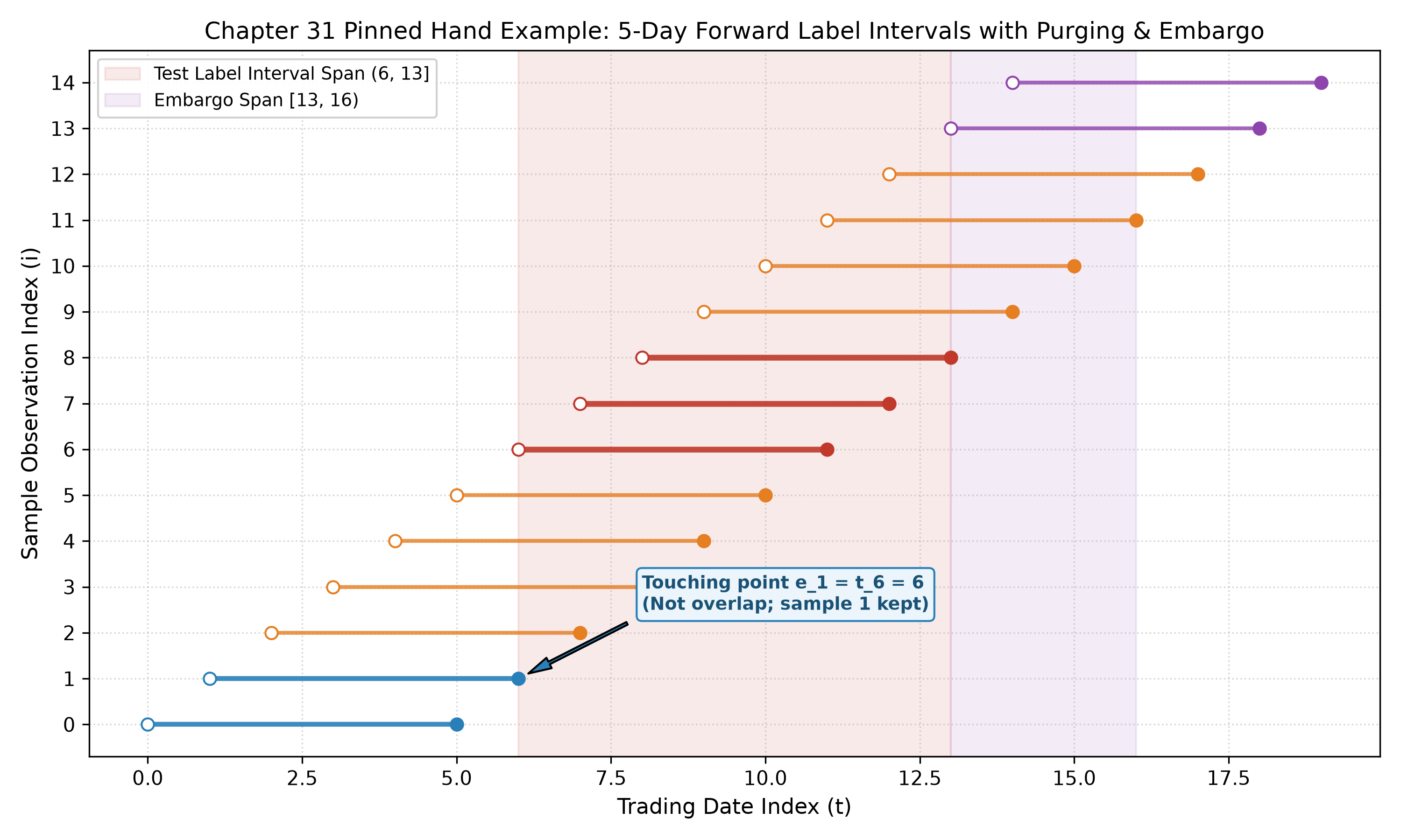
• File path: figures/a6/ch31_hand_label_intervals.png.
• Axes and units: The horizontal axis is the shared observation position $t$ (a discrete integer extending through the final label endpoint, 19; 15 label starts do not mean the labels end at 14). The vertical axis is the sample observation index $i$ (integer, 0 to 14).
• Samples and marks: All 15 half-open return intervals $(t,t+5]$ are shown. Left endpoints are hollow circles and right endpoints are filled circles. Test-block samples $\{6,7,8\}$ are thick dark-red lines; samples $\{2,3,4,5,9,10,11,12\}$ removed by Purge for overlapping labels are orange; samples $\{13,14\}$ removed by Embargo for feature lookback penetration are purple; and the final clean training samples $\{0,1\}$ are thick dark-blue lines.
• What to look for:
  1. The filled right endpoint of sample 1's label interval $(1,6]$ coincides exactly at $t=6$ with the hollow left endpoint of test sample 6's interval $(6,11]$. An arrow labels this “Endpoint touch, not overlap (touching point $e_1=t_6=6)$,” showing why sample 1 is safely retained.
  2. The label interval for post-test sample $t=13$ does not overlap the test block, but it falls inside the purple embargo span $[13,16)$, showing how Embargo protects against feature lookback.

10.2 Leakage Ablation Comparison and Breakdown

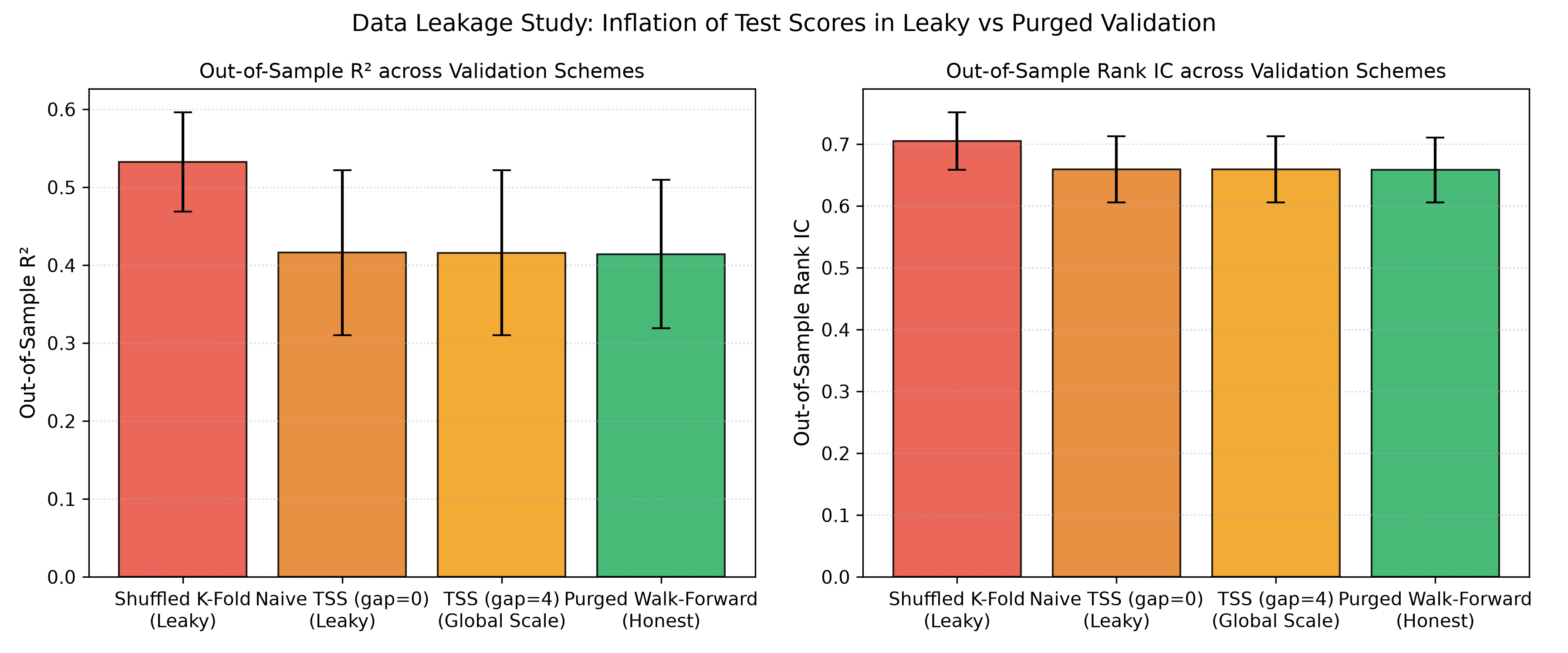
• File path: figures/a6/ch31_leakage_comparison.png.
• Axes and units: The left panel shows out-of-sample coefficient of determination $R^2$ (dimensionless); the right panel shows out-of-sample rank correlation, Rank IC (dimensionless). The horizontal axis compares four validation schemes. Error bars show the standard deviation across five random seeds ([20261031, 20261032, 20261033, 20261034, 20261035]).

The table reports the observed five-seed mean values (key: leakage_experiment.schemes):

• What the comparison shows:
  1. Observed differences between protocols: The saved mean $R^2$ difference between Shuffled K-Fold and Purged Walk-Forward is 0.1184 (the Rank IC difference is 0.0471). The gap between the first two schemes is 0.1167, while the gap between the latter two protocols is about 0.0017. These are not matched ablations: Shuffled K-Fold and TSS use different training dates and sample sizes, while TSS and Purged Walk-Forward also differ in date grouping, Purge, and scaling range. The value 0.1167/0.1184, or about 98.6%, cannot be called a causal share attributable to shuffling; nor can 0.0017 be attributed to Purge alone. Identifying the contribution of any one change requires matching the training samples, test samples, preprocessing, and other conditions.
  2. Boundary effects in the current linear-model comparison: In this Ridge construction with 20 assets, 500 days, and five seeds, the four-day label overlap at the boundaries of five large test blocks (80 days each) accounts for less than 2% of the training samples. The observed scores before and after purging are close. This describes the current design only; it does not show that low-capacity models are generally unaffected by leakage or that leakage effects occur only in high-capacity models or particular features.
  3. Unpurged inflation with a high-capacity memorization model (1-NN): To illustrate how label overlap can affect a high-capacity memorization model, a 1-nearest-neighbor (1-NN) model was evaluated in daily forward steps on a 30-asset panel (key: overlap_memorization_experiment).
     • The unpurged 1-NN model had a mean out-of-sample Rank IC of $0.1194$ (the five seeds were $0.0977$, $0.0942$, $0.1691$, $0.1109$, and $0.1249$).
     • The causal Purged result had a mean Rank IC of $0.0108$ (the five seeds were $0.0007$, $-0.0189$, $0.0784$, $0.0061$, and $-0.0121$). These are observations under this data-generating process and a finite set of seeds, not a guarantee about true population predictive power.
     • In this construction, the unpurged model can match a test asset to its own unpurged sample from the previous day; the two labels share 80% of their returns. The five-seed mean Rank IC difference is $0.1086$ (key: overlap_memorization_experiment.rank_ic_inflation). This shows how some highly memorizing models may exploit label overlap. Together with the Ridge result, it does not establish a general monotonic relationship between model capacity and leakage bias.

10.3 Comparison of Row-Count gap with Interval Purge

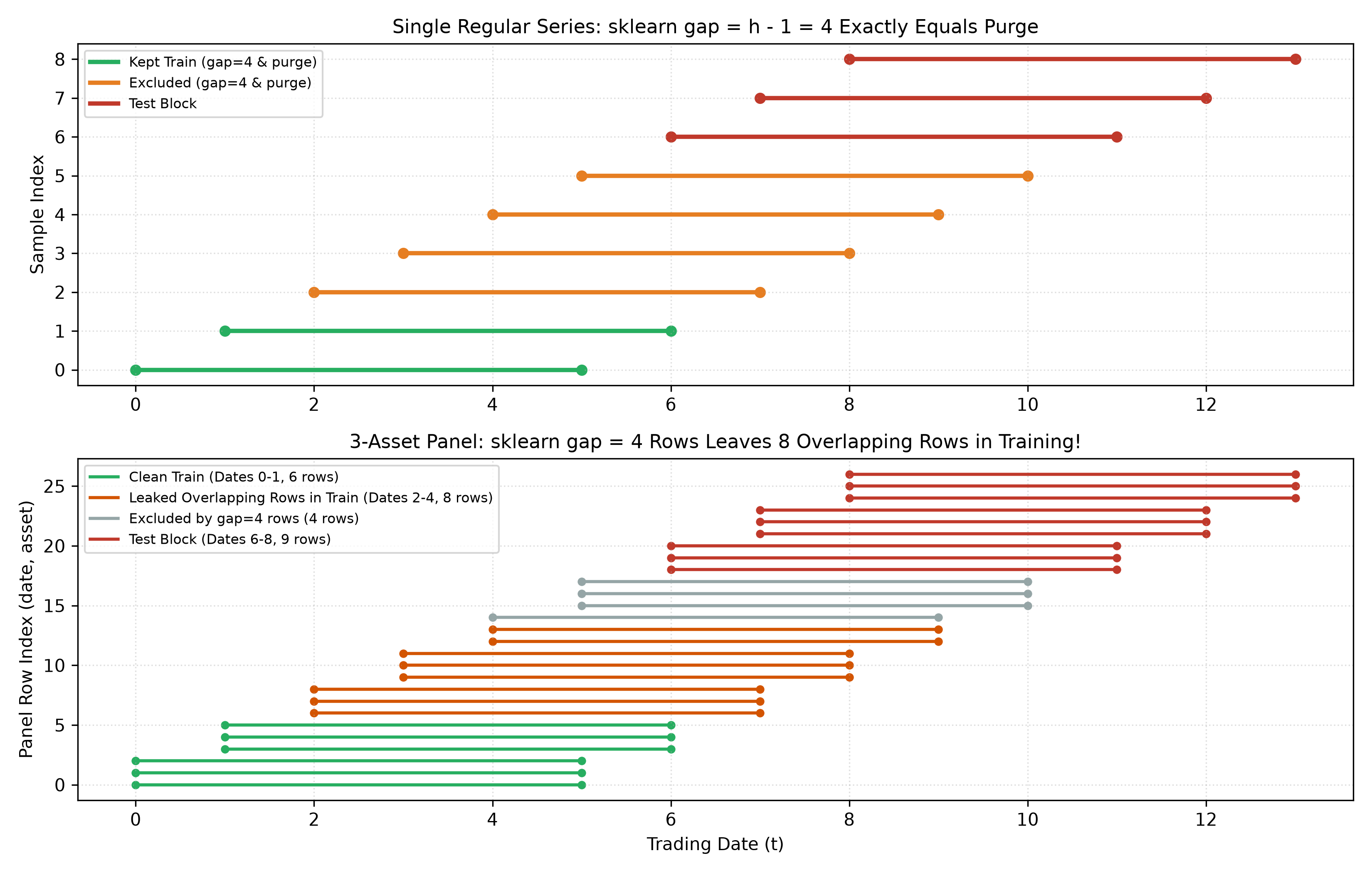
• File path: figures/a6/ch31_gap_vs_purge_panel.png.
• Axes and units: The upper panel shows a single-asset sequence (sample indices 0–8); the lower panel shows a three-asset panel (row indices 0–26, ordered by (date, asset)). Both horizontal axes show trading-day index $t$.
• What to look for:
  1. In the single-asset sequence, gap=4 removes samples 2, 3, 4, and 5, exactly matching Purge row by row.
  2. The panel-data plot shows the substantial residual overlap: gap=4 removes only rows 14–17 (gray), while rows 6–13 (dark orange, covering eight rows across dates 2, 3, and 4) remain exposed in the training set, visually confirming Theorem 2.

10.4 Mean-Summary Plot for Rolling Validation on Real Monthly Industry Returns

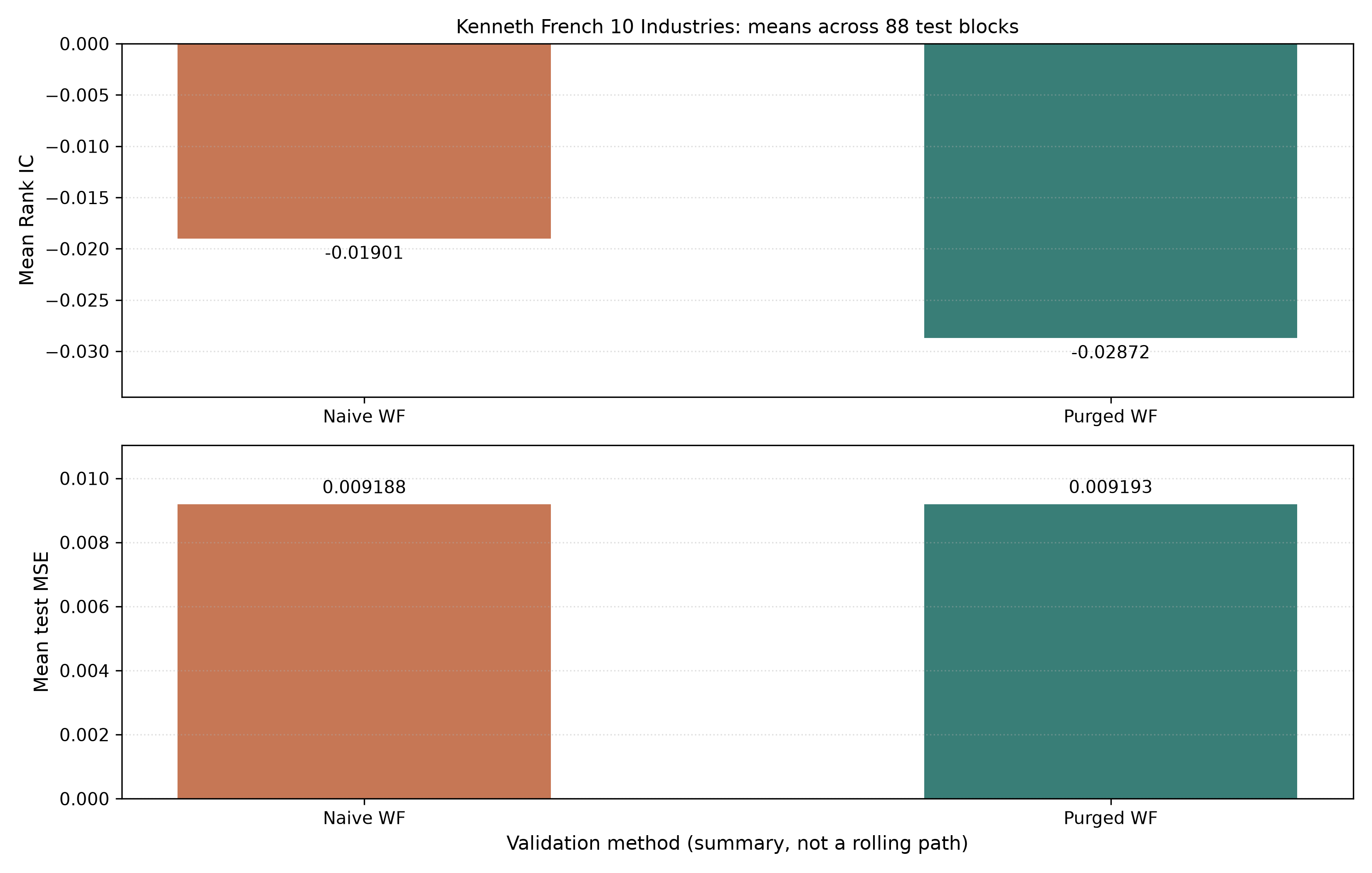
• File path: figures/a6/ch31_french_rolling_validation.png.
• Axes and units: The horizontal axis compares naive and purged validation. The upper panel shows mean Rank IC across 88 test blocks; the lower panel shows mean test MSE. Bar heights show only the saved summary means. They do not show the block-level paths, stability across blocks, or statistical significance of the method difference.
• What to look for:
  1. With three-month forward overlapping labels, mean test MSE is $0.009188$ for naive Walk-Forward and $0.009193$ for Purged Walk-Forward.
  2. On the real academic aggregate industry data, the observed mean Rank IC is $-0.01901$ and $-0.02872$, respectively. The experiment reports no uncertainty for these means and no significance test, so the negative means do not establish that positive Alpha is absent in the population. The figure reports only the observed results for this dataset, model, and validation window.

11. Real-Market Example

This section preserves a historical methodological illustration; it is not a newly acquired dataset or rerun. Raw, extracted, and processed French files are absent from the default I3 package, whose Notebook skips this branch. Rights, subjects, and intended uses need separate review. A10-A/A10-A.1 do not replace G05/A10-B execution authorization.

To illustrate model validation on real-market assets, we use the frozen Kenneth R. French 10 Industry Portfolios monthly total-return data in the workspace, covering 1926-07 through 2026-08 (1,202 monthly observations).

11.1 Data Properties and Scope

• Sources: Kenneth R. French Data Library: 10 Industry Portfolios (value-weighted, monthly) and the FF3 risk-free rate (RF).
• Files and hash verification:
  • Data manifest: data/manifests/french_industries_2026-10-05.json (SHA-256: 3b71cd5f781f9790cc380195c22635e03e9c9e27a5f43cd2d0d46fb12efa8271).
  • Processed return table: data/processed/french_10_industries_monthly.csv (SHA-256: 3b097d810c295d64eedfa1ece7067ff2a0707f5ca90e33935df9949251f70950).
• Academic-use and tradability boundaries: These data are academic aggregate portfolios, have been revised historically, and are not point-in-time snapshots (is_point_in_time: false). They also do not represent the tradable liquidity of individual securities. This example therefore supports methodological instruction only and does not make a live-trading Alpha claim.

11.2 Design: Three-Month Overlapping Forward Returns and Rolling Validation

• Prediction target: Three-month compounded forward return ($h=3$):

  $$y_{i,t}=\prod_{k=1}^3(1+R_{i,t+k})-1$$

• Feature engineering:

  • 12-month trailing momentum: $X_{0,i,t}=\prod_{k=0}^{11}(1+R_{i,t-k})-1$.
  • One-month short-term reversal: $X_{1,i,t}=R_{i,t}$.

• Rolling Walk-Forward windows:

  • Fixed training window: 120 months (10 years).
  • Test block: 12 months (1 year).
  • Step size: 12 months (annual tuning).
  • The full sample produces 88 non-overlapping 12-month calendar test blocks. Forward labels can still overlap across blocks, so the blocks are not necessarily statistically independent (key: french_market_experiment.eval_blocks).

• Protocol comparison:

  1. Naive Walk-Forward: The training set consists of the 120 months immediately before each test block, with no Purge. The return intervals for the final two training labels, $y_{t-1}$ and $y_{t-2}$, extend into the first two months of the test block.
  2. Purged Walk-Forward: Purge removes the two months at the end of the training set whose return intervals overlap the test set.

11.3 Observed Results and Reconciliation

The table reports CLI results preserved in an earlier independent review; they were not rerun for this revision (build/codex_a6/final_learning_review/ch31/recheck/results/ch31_results.json):

Interpretation:

1. With a 120-month training sample and only two months of overlap (1.67% of the training window), the out-of-sample MSE values are very close: $0.009188$ versus $0.009193$.
2. The mean out-of-sample Rank IC is slightly negative for both schemes in this split ($-0.01901$ and $-0.02872$). The table provides no standard errors, confidence intervals, or test. It supports reporting these sample means only; it does not establish that the population relationship is negative, statistically insignificant, or devoid of Alpha. These academic aggregate portfolios also do not support a tradability conclusion.

12. Common Mistakes

12.1 Mistake 1: Using Randomly Shuffled K-Fold as the Default for Financial Time Series

• Incorrect example and why it fails: This ignores time order and the label-dependence window. After shuffling, adjacent samples can appear in both the training and test sets. When their label windows share information, the test score may be optimistic; the magnitude depends on the data-generating process, features, model, and split. The code below is a fixed synthetic counterexample and does not establish a general bias magnitude.
• Runnable comparison code:

import numpy as np
from sklearn.linear_model import Ridge
from sklearn.model_selection import KFold
from quant_course.validation import walk_forward_splits

rng = np.random.RandomState(42)
N, h = 100, 5
X_all = rng.randn(N + h - 1, 2)
X = X_all[:N]
# period_returns[k] belongs to (k,k+1], so y[i] settles at i+h.
period_returns = 0.6 * X_all[:, 0] + rng.normal(0, 0.2, len(X_all))
y = np.array([period_returns[i:i+h].sum() for i in range(N)])
t = np.arange(N, dtype=float)
e = t + h
a = e.copy()
kf = KFold(n_splits=5, shuffle=True, random_state=42)
scores_leaky = [Ridge().fit(X[tr], y[tr]).score(X[te], y[te]) for tr, te in kf.split(X)]
splits = walk_forward_splits(N, 50, 10, step=10, t=t, e=e)
scores_forward = []
for tr, te in splits:
    tr = tr[a[tr] <= t[te].min()]
    assert np.all(e[tr] <= t[te].min())
    scores_forward.append(Ridge().fit(X[tr], y[tr]).score(X[te], y[te]))
assert np.isfinite(scores_leaky).all() and np.isfinite(scores_forward).all()
print("Shuffled / forward:", np.mean(scores_leaky), np.mean(scores_forward))

The old centered convolution, convolve(X, ones(5)/5, mode="same"), depends on $X_{t-2},\ldots,X_{t+2}$ at interior points. Labeling it as $(t,t+5]$ does not describe its true support, and matching the interval length to five does not fix the metadata. This example instead uses an explicit forward array: each label $i$ sums five synthetic returns over $(i,i+1],\ldots,(i+4,i+5]$, with $e_i=a_i=i+5$. Future $X$ values are used only to generate future returns, not as features available at the prediction time. This is a new small teaching example, not the saved five-seed study below, and it does not assert that shuffled scores must be higher on every sample.

• Observed score differences: In the five-seed synthetic panel study, the four schemes had the following results:
  1. Shuffled K-Fold: mean $R^2=0.5327$ (Rank IC $=0.7054$).
  2. Naive TSS (gap=0): $R^2=0.4160$ (Rank IC $=0.6593$).
  3. TSS (gap=4, global normalization): $R^2=0.4160$ (Rank IC $=0.6594$).
  4. Causal Purged Walk-Forward: $R^2=0.4143$ (Rank IC $=0.6583$). In this linear Ridge construction, the $R^2$ difference between Shuffled K-Fold and Purged Walk-Forward is $0.1184$. The observed difference between the first two protocols is $0.1167$, and the difference between TSS and the final protocol is about $0.0017$. Because the training/test blocks, samples, and preprocessing all differ, these values do not support a one-factor causal decomposition. In a separate 1-NN construction, the mean Rank IC was $0.1194$ without Purge and $0.0108$ with Purge (a difference of $0.1086$). These are simulation results under their respective designs, not general laws about model capacity, leakage, or bias magnitude.

12.2 Mistake 2: Treating TimeSeriesSplit's gap as a Number of Days in a Multi-Asset Panel

• Incorrect example: On a daily panel of 20 stocks, a researcher predicts five-day forward returns and assumes that TimeSeriesSplit(gap=4) removes four days.
• Why it fails: TimeSeriesSplit's gap parameter counts sample rows, not dates. In a 20-stock panel, gap=4 removes only four rows, less than one trading day's records; more than three days of overlapping data remain leaked.
• Fix: Use quant_course.validation.purge to filter explicitly by the trading-date array, or derive indices from unique dates before calling TimeSeriesSplit.
• Numerical difference: In the three-asset example, gap=4 left eight overlapping rows in the training set.

12.3 Mistake 3: Normalizing Features on the Full Sample Before Splitting

• Why it fails: Future test-set means and extreme values are incorporated into the full feature matrix, so the training features use a baseline containing information about the test period's structure.
• Runnable comparison code:

import numpy as np
from sklearn.preprocessing import StandardScaler

rng = np.random.RandomState(42)
X = rng.randn(100, 2) + 2.0

# Incorrect: normalize on the full sample
X_scaled_all = StandardScaler().fit_transform(X)
X_test_leaky = X_scaled_all[80:]

# Correct: fit on the training set only
scaler = StandardScaler()
X_train_clean = scaler.fit_transform(X[:80])
X_test_clean = scaler.transform(X[80:])

# Check that the two transformations differ
assert not np.allclose(X_test_leaky, X_test_clean)

• Observed score difference: Fitting the scaler globally brings test-period distribution information into the training feature baseline. In this small example, the two transformations differ, but the direction of any estimated volatility or mean-drift error is not guaranteed for every sample.

12.4 Mistake 4: Applying Embargo to Training Samples Before the Test Block

• Why it fails: This misunderstands the causal role of Embargo. Embargo guards against backward-looking features reaching into the test labels and is therefore necessary only for training samples located after the test block. Under this chapter's post-test definition, a purely historical forward split has no post-test candidates, so the embargo-removal set is empty. Historical dependency gaps or feature warm-up periods for other purposes are separate constraints; this point does not rule them out.
• Fix: In code, require is_after_test = t_i >= t_test_max and apply the interval filter $[e_{\max},e_{\max}+m)$ only to samples satisfying that condition.

12.5 Mistake 5: Treating Endpoint Touching as Overlap and Removing Too Many Samples

• Incorrect interpretation: A researcher assumes there is overlap when one sample settles at the close on day 6 and the test prediction starts after the close on day 6.
• Economic meaning: The earlier label's return ends at $r_6$, while the later label begins at $r_7$, so the half-open intervals have an empty intersection. Sharing a reference closing price does not mean the price is non-random, nor does it imply that the two returns are statistically independent. The actual order of close settlement, data ingestion, and prediction must still be checked against the event clock; endpoint contact alone does not establish that those events were ordered correctly.

13. Quant Research Application

13.1 End-to-End Validation Pipeline for Quantitative Research

In industry quantitative research, an immutable, leakage-resistant model-validation process is a core safeguard in strategy development. A standard pipeline has four stages:

Stage 1: Freeze the protocol and plan (Ch 22 ResearchPlan)
    - Specify the primary metric (Rank IC), test horizon h, maximum feature lookback m, and asset universe.
Stage 2: Define sample intervals and construct labels (Ch 3, 31)
    - Record each sample's observation time t_i, label end e_i, and availability time a_i.
    - At each prediction time, first filter for a_i <= t_predict; the current helper performs interval Purge using (t_i, e_i) only.
Stage 3: Run the outer causal Walk-Forward (Outer Purged Walk-Forward)
    - Set a historical training window; check a-eligibility and then label overlap. In a purely historical forward split, the post-test Embargo set is empty.
Stage 4: Select hyperparameters in nested inner folds (Inner Nested Selection)
    - Generate subfolds only within the current outer training set; fit normalization only on each inner training set.

13.2 Practical Falsification Rules and Negative Criteria

After building the validation pipeline, a quantitative team should run the following falsification checks:

1. Future Invariance Test: With random seeds, identifiers and column schema, and algorithm policy held fixed, apply specified perturbations to valid future inputs and compare model parameters and hyperparameters at shared historical coordinates. Differences beyond the declared tolerance warrant investigation for leakage or nondeterminism. Passing this finite set of tests does not establish validity under every future change or the legality of all input timestamps.
2. Shuffling Ablation Check: Compare Purged Walk-Forward with shuffled K-Fold. Similar or reversed scores alone do not establish a lack of temporal dependence or model underfitting; a large difference alone cannot be attributed uniquely to label memorization. First match the evaluation target, training/test dates and sample sizes, and preprocessing. Then investigate distribution and feature support, while preserving results from every protocol.

14. Chapter Summary

14.1 Conceptual Flow

First choose the purpose: historical deployment with available labels, or offline diagnosis with future blocks.
Candidate C -> Does its label overlap?
  Yes -> R_purge: remove the sample and terminate this branch.
  No -> S_after_purge -> Is it post-test and inside the buffer?
    Yes -> R_embargo: remove the sample and terminate this branch.
    No -> S_final -> Scale and select separately within each inner and outer fold.

Neither removal node has an outgoing edge. Only $S_{\mathrm{after\_purge}}$ proceeds to the Embargo check; there is no path back from either removal set to the final set. Choose the deployment or diagnostic branch before generating candidates. Filtering cannot turn a future training block into a deployment split. Fit the scaler and tune within the training folds after filtering, applying the interval rules separately in the inner and outer folds.

For a numerical walk-through of the diagram, sample 2 overlaps and enters $R_{\mathrm{purge}}$, where its branch ends. Sample 1 touches an endpoint, passes through the no-overlap branch to $S_{\mathrm{after\_purge}}$, and enters $S_{\mathrm{final}}$ because it is before the test block. Sample 13 also passes Purge because it only touches an endpoint, but its observation time falls in $[13,16)$, so it enters $R_{\mathrm{embargo}}$ and its branch ends. Calling both removed and surviving sets “purged” would hide the direction that matters most.

14.2 Decision Rules for Validation Schemes

Researchers should choose a validation architecture according to the research question:

15. Exercises

31-E01: Testing for Overlap Between Half-Open Label Intervals

For one asset's daily data, three samples have the following time parameters:

• Sample A: $t_A=2,\ e_A=6$.
• Sample B: $t_B=5,\ e_B=9$.
• Sample C: $t_C=6,\ e_C=10$.

Determine:

1. Do samples A and B overlap? Give their intersection.
2. Do samples A and C overlap? Explain why or why not.

31-E02: Purge Sample Count on a Regular Single-Asset Calendar

A single-asset trading calendar is continuous and has no missing observations. The forecast holding period is $h=10$ trading days. If the test set starts at trading-day index $t=100$, derive the index range of training samples before the test set that Purge removes, and give the total number of samples.

31-E03: Why Embargo Is Not Needed in a Purely Forward Split

Why does a purely forward Walk-Forward split, in which every training sample occurs before the test block, require Purge but no Embargo? Prove this from the perspective of causal information flow and the mathematics of feature lookback windows.

31-E04: Availability Later Than Label Settlement

A factor label is based on a listed company's quarterly return on equity (ROE). Assume the fiscal quarter ends at $e_i=\text{2025-03-31}$, but the actual publication and ingestion time is $a_i=\text{2025-04-30 10:00}$. This is a fact stipulated by the exercise, not inferred from a statutory filing deadline.

If the model prediction time is $t_{\text{predict}}=\text{2025-04-15 15:00}$, may this sample enter the current training set? What bias would arise if it were used as a training sample on 2025-04-15?

31-N01: Find the “Resurrected Sample” in the Flowchart (New)

Someone connects “overlap → remove by Purge” to “not post-test → retain,” then adds the retained item to the final training set. Use sample 2 to explain the error and write the four correct sets with their containment relationships. Explain why samples 1 and 13, which both touch endpoints, have different final outcomes. If the deployment time is 6 and sample 1 has $a_1=7$, at which gate should it be blocked?

16. Programming Exercises

31-P01: Implement a Half-Open Interval Intersection Test

Write a function is_overlapping(t1: float, e1: float, t2: float, e2: float) -> bool and verify that it:

1. Raises ValueError when an input has $e\le t$.
2. Correctly returns whether the half-open intervals $(t_1,e_1]$ and $(t_2,e_2]$ intersect.
3. Returns False for the endpoint-touching pair $(1,6]$ and $(6,11]$.

31-P02: Implement Purge for a Cross-Sectional Panel

Write a function panel_purge(train_dates: np.ndarray, test_dates: np.ndarray, h: int) -> np.ndarray. The inputs are row-date arrays from a five-asset panel, with multiple rows on the same date. The test set contains samples from specified dates. Return the row indices retained in the training set after Purge, and assert that no observations on overlapping dates remain.

31-P03: Demonstrate the Failure of scikit-learn TimeSeriesSplit gap

Write a standalone Python script that constructs a synthetic panel with three assets over 15 trading days, uses labels with $h=5$ days, and sets dates 6–8 as the test set. Run TimeSeriesSplit(gap=4), calculate the number of overlapping rows left in training exactly, and verify whether it is exactly eight.

31-P04: Implement a Strictly Leakage-Resistant Nested Evaluator

Using sklearn.linear_model.Ridge, implement a hyperparameter selector with two outer causal forward folds and two inner validation folds. Fit feature-scaling parameters only on the inner training set, and report the uncontaminated mean squared error on the outer test sets.

17. Challenge Problems

31-C01: Purge Interval Algebra for Irregular Calendars and Suspended Assets (Open Derivation)

In real A-share or Hong Kong markets, an asset may be suspended for several weeks, or different assets may use different delivery and settlement calendars.

1. Formally define label intervals that incorporate each asset's individual suspension calendar.
2. Prove that, on an irregular calendar, the simplified addition $e_i=t_i+h$ based on trading-day index $t$ can cause local lookahead or over-purge.
3. Propose a rubric for designing a robust Purge engine aligned by actual calendar days or tradable tick timestamps.

31-C02: A Counterexample to Purged K-Fold Under a Nonstationary Regime Shift (Theory and Numbers)

Construct a two-stage Markov regime-switching data-generating process, such as a low-volatility bull market followed by a high-volatility bear market.

Show that even if Purged K-Fold completely removes overlapping labels and feature-embargo leakage, training on future bear-market data while testing a historical bull-market interval can still make the model parameters differ substantially from the parameters best for the historical regime. Give quantitative evidence and recommendations.

31-C03: Purged Validation Gates Combined with a Multiple-Testing Trial Ledger (Integrated Design)

Combine the TrialLedger from Chapter 22 with the future-perturbation test from Chapter 30 to design an integrated quantitative strategy-admission verification protocol. The protocol must record the Purged splits used to evaluate every hyperparameter variant, account for the number of effective independent trials, and retain a final holdout-test safeguard.

31-C04: Extending Validation to Continuous Labels and Event-Driven Triple-Barrier Labels

Financial applications often use take-profit, stop-loss, and time-expiry triple-barrier labels, in which the label end time $e_i$ is a random variable triggered by the price path.

Derive and prove that, under triple-barrier labeling, each sample's $e_i$ is no longer a constant $t_i+h$. Explain how to compute variable-length Purge and Embargo sets dynamically.

18. Solutions and Solution Hints

31-E01 Solution

1. Samples A and B:
   • Sample A has interval $I_A=(2,6]$, and sample B has interval $I_B=(5,9]$.
   • For the overlap test, $\max(t_A,t_B)=\max(2,5)=5$ and $\min(e_A,e_B)=\min(6,9)=6$.
   • Since $\max(t_A,t_B)=5<\min(e_A,e_B)=6$, the samples overlap.
   • Their intersection is $(\max(t_A,t_B),\min(e_A,e_B)]=(5,6]$.
2. Samples A and C:
   • Sample A has interval $I_A=(2,6]$, and sample C has interval $I_C=(6,10]$.
   • The overlap test gives $\max(t_A,t_C)=\max(2,6)=6$ and $\min(e_A,e_C)=\min(6,10)=6$.
   • The condition $\max(t_A,t_C)<\min(e_A,e_C)$ does not hold, because $6<6$ is false. The samples do not overlap.
   • Economically, sample A's return settles at the close on day 6, while sample C's return starts after the close on day 6. They touch at one endpoint on the time axis but share no holding-period return.

31-E02 Solution

• As derived in §6.2, when the test block starts at $t_{\text{test}}=100$, its first sample has interval $(100,100+10]=(100,110]$.

• A historical training sample at $t_i$ has interval $(t_i,t_i+10]$.

• The necessary and sufficient condition for overlap with the test set is $t_i+10>100\iff t_i>90$.

• Since $t_i<100$, the exact range of historical training indices removed by Purge is:

  $$t_i\in\{91,92,93,94,95,96,97,98,99\}$$

• The total removed is $99-91+1=9=h-1$ samples.

31-E03 Solution

• Proof:
  1. Embargo is defined to prevent the feature lookback window of post-test training samples from reaching into the test set's realized-return label intervals.
  2. In a purely forward Walk-Forward split, every training sample satisfies $t_{\text{train}}<t_{\text{test},\min}$.
  3. When historical training features are calculated from technical indicators or rolling features, they use information from earlier times, at indices $\le t_{\text{train}}<t_{\text{test},\min}$. They lie entirely before the test set.
  4. Historical training features therefore cannot, in the causal time order, reach into the future test interval.
  5. Thus a purely forward training set has no feature-lookback penetration risk. Purge is still needed to remove label overlap at the end of the training set, but Embargo is not needed.

31-E04 Solution

• Decision: This sample must not enter the current training set.
• Reason and bias:
  • Although the operating period reflected by the financial statement ended at $e_i=\text{2025-03-31}$, at the model decision time $t_{\text{predict}}=\text{2025-04-15 15:00}$ the stipulated actual availability time is April 30 at 10:00. The statement is not yet readable on April 15 at 15:00. If only the statutory latest filing deadline were known, without the actual publication and ingestion time, that would not establish whether the information was unknown on April 15; the actual timestamp would need to be checked.
  • Treating the sample as known training data on April 15 would fit model parameters using information that had not yet been disclosed, creating classic look-ahead bias.
  • The correct condition for a sample to enter training is the availability-time constraint $a_i\le t_{\text{predict}}$.

31-N01 Full Solution (New)

The interval $I_2=(2,7]$ for sample 2 overlaps $I_6=(6,11]$, so sample 2 must be removed. “Not post-test” can determine whether a candidate that has not already been removed is exempt from Embargo; it cannot restore a sample removed by Purge. The sets are $R_{\mathrm{purge}}=\{2,3,4,5,9,10,11,12\}$, $S_{\mathrm{after\_purge}}=\{0,1,13,14\}$, $R_{\mathrm{embargo}}=\{13,14\}$, and $S_{\mathrm{final}}=\{0,1\}$. The final set is contained in the Purge survivors, which are contained in the candidate set.

The return set for sample 1 ends at $r_6$, while sample 6's begins at $r_7$. The return set for sample 13 begins at $r_{14}$, while sample 8's ends at $r_{13}$. Neither pair overlaps. Sample 13 is in the post-test buffer $[13,16)$, however, so its feature lookback reaches into the test labels and it must be embargoed. If $a_1=7>6$, sample 1 should be removed before deployment candidates are generated, not left for the interval-touching test to decide.

31-P01 Reference Implementation

def is_overlapping(t1: float, e1: float, t2: float, e2: float) -> bool:
    if e1 <= t1 or e2 <= t2:
        raise ValueError("Label end e must be strictly greater than observation time t")
    return max(t1, t2) < min(e1, e2)

# Test assertions
assert is_overlapping(2, 7, 6, 11) is True
assert is_overlapping(1, 6, 6, 11) is False  # Endpoint touching is not overlap
assert is_overlapping(0, 5, 6, 11) is False

31-P02 Reference Implementation

import numpy as np
from quant_course.validation import purge

def panel_purge(train_dates: np.ndarray, test_dates: np.ndarray, h: int) -> np.ndarray:
    # Dates are common integer observation positions, not datetime strings.
    if isinstance(h, bool) or h < 1 or int(h) != h:
        raise ValueError("h must be a positive integer observation horizon")
    e_train = train_dates + float(h)
    e_test = test_dates + float(h)
    cand_idx = np.arange(len(train_dates))
    test_idx = np.arange(len(test_dates))
    # Concatenate the full sample for the standard purge
    all_t = np.concatenate([train_dates, test_dates])
    all_e = np.concatenate([e_train, e_test])
    test_offset_idx = np.arange(len(train_dates), len(all_t))
    purged = purge(cand_idx, test_offset_idx, all_t, all_e)
    return purged

# Verification
dates_tr = np.repeat(np.arange(6), 5)  # Five assets on every date 0..5.
dates_te = np.repeat(np.array([6, 7, 8]), 5)
kept = panel_purge(dates_tr, dates_te, h=5)
assert np.array_equal(kept, np.arange(10))  # dates 0 and 1: all ten rows
assert not np.any(np.maximum(dates_tr[kept, None], dates_te[None, :]) <
                  np.minimum(dates_tr[kept, None] + 5, dates_te[None, :] + 5))

31-P03 Reference Implementation

import numpy as np
from sklearn.model_selection import TimeSeriesSplit

dates = np.repeat(np.arange(15), 3)  # 45 rows
test_idx = np.arange(18, 27)         # dates 6..8, 9 rows total
tss = TimeSeriesSplit(n_splits=3, test_size=9, gap=4)
train_tss, test_tss = next(tss.split(np.arange(45)))
assert np.array_equal(test_tss, test_idx)  # Full 45-row sample: first test rows 18..26
assert np.array_equal(train_tss, np.arange(14))
e = dates + 5
overlapping_rows = [i for i in train_tss if any(
    max(dates[i], dates[j]) < min(e[i], e[j]) for j in test_tss)]
assert overlapping_rows == list(range(6, 14))
print("Overlapping rows left in training:", len(overlapping_rows))
assert len(overlapping_rows) == 8

31-P04 Reference Implementation

The forward array period_returns[i] represents the return over $(i,i+1]$, corresponding to the formal notation $r_{i+1}$. The label y[i] is the sum of the next two returns, with $e_i=a_i=i+2$. Future array values generate the label and must not enter the current feature vector. Each outer fold has two distinct inner validation windows. Each uses only earlier training rows whose labels are available; the helper then applies Purge, and scaling is fit only on that training fold.

import numpy as np
from sklearn.linear_model import Ridge
from quant_course.validation import nested_hyperparameter_evaluation

rng = np.random.RandomState(123)
N = 100
X_all = rng.randn(N + 1, 2)
X = X_all[:-1]
period_returns = 1.2 * X_all[:, 0] + rng.randn(N + 1) * 0.2
y = period_returns[:-1] + period_returns[1:]
t = np.arange(N, dtype=float)
e = t + 2.0
a = e.copy()  # Availability equals interval end in this example.

candidate_splits = [(np.arange(50), np.arange(50, 75)), (np.arange(75), np.arange(75, 100))]
outer_splits = []
for train_idx, val_idx in candidate_splits:
    prediction_time = np.min(t[val_idx])
    outer_splits.append((train_idx[a[train_idx] <= prediction_time], val_idx))
def inner_split(out_tr, t_arr, e_arr):
    n = len(out_tr)
    folds = []
    for start, stop in [(n // 3, 2 * n // 3), (2 * n // 3, n)]:
        in_train = np.arange(start)
        in_val = np.arange(start, stop)
        prediction_time = np.min(t_arr[out_tr[in_val]])
        in_train = in_train[a[out_tr[in_train]] <= prediction_time]
        folds.append((in_train, in_val))
    return folds

res = nested_hyperparameter_evaluation(
    X, y, t, e, outer_splits, inner_split,
    [{"alpha": 0.1}, {"alpha": 10.0}],
    lambda p: Ridge(alpha=p["alpha"]),
    lambda m, Xt, yt: -float(np.mean((m.predict(Xt) - yt) ** 2)),
    scale_features=True
)
assert len(res["outer_scores"]) == 2
assert all(len(folds) == 2 for folds in res["inner_splits_used"])
for folds in res["inner_splits_used"]:
    for fold in folds:
        tr = np.array(fold["train_idx"]); va = np.array(fold["val_idx"])
        assert tr.size and va.size and t[tr].max() < t[va].min()
        assert np.all(a[tr] <= t[va].min())
        assert not np.any(np.maximum(t[tr, None], t[None, va]) <
                          np.minimum(e[tr, None], e[None, va]))
print("Outer MSE:", [-s for s in res["outer_scores"]])
print("Purged outer splits:", res["outer_splits_used"])
print("Purged inner splits:", res["inner_splits_used"])

31-C01 Full Reference Answer: Irregular Calendars

First state the economic target. This problem defines settlement as the next two valid price observations for that asset, not the next two calendar days. A real study could instead use a fixed common-calendar horizon; those are different labels and should not be treated as interchangeable. Let $\tau_i(t,2)$ return the second valid observation date for asset $i$ after $t$. Asset A has observable dates $0,1,2,8,9,10$, with no executable price during its suspension; asset B is observable every day. A's label at $t=2$ ends at $e=9$, giving interval $(2,9]$. B's label at $t=2$ ends at $4$, giving interval $(2,4]$. Let the test sample be $(8,10]$. Check each interval:

Thus A and the test interval share $(8,9]$, so A must be purged. For B, the condition $8<4$ is false, so B is retained. If A's end were incorrectly set to $2+2=4$, the true overlap would be missed. Training eligibility also requires the actual label-availability time $a_i\le t_{\mathrm{predict}}$; a post-suspension settlement value cannot be available in advance. All intervals here remain half-open, so endpoint touching is not overlap.

For precise Purge, use the actual end time $e_i=\tau_i(t_i,h)$ for every row. A training sample is retained only if:

This is the requirement that it not overlap any test sample, rather than a check against an arbitrary representative date. If a single conservative endpoint is required, take $e^{\max}(t)=\max_i e_i(t)$ across assets on the same date and purge against $(t,e^{\max}(t)]$. This envelope contains each actual interval, so it will not miss an overlap, but it may wrongly remove B's non-overlapping training sample in this example and reduce the usable sample size. A longer interval does not provide more information. Report the difference between the conservative and precise rules.

31-C02 Full Reference Answer: Purging Does Not Remove Mechanism Changes

First define a two-state Markov chain with $S_0=0$ and transition matrix $\begin{pmatrix}1-p&p\\0&1\end{pmatrix}$, where $0<p<1$. Consider the path $S_0,\ldots,S_{2m-1}=0$ and $S_{2m},\ldots,S_{3m-1}=1$. Its probability is $(1-p)^{2m-1}p>0$. This is a positive-probability path under an absorbing two-stage mechanism; it does not imply the same error on every realization or every path.

Sample $i$ is formed at $i-1$. Its one-period label $y_i=2S_i$ settles at $i$ and is then available, with interval $I_i=(i-1,i]$. The endpoint is settled before fitting at the same timestamp. Divide the path into three equal contiguous blocks, B0, B1, and B2, each with $m$ labels. Labels are 0 in B0 and B1, and 2 in B2. The adjacent return intervals at block boundaries only touch, so correct Purge does not change the following training sets.

For a bidirectional K-Fold test on B0, train on B1 and B2. The training-label mean is $(0+2)/2=1$, so the B0 test MSE is $(0-1)^2=1$. But at the historical B0 time, B2 has not yet occurred; this model is not a deployable historical prediction. Under strict forward validation, train on B0 and test on B1. The training mean is 0 and the MSE is 0. When B2 is the first block after the regime change, training on B0 and B1 still predicts 0, giving B2 test MSE $(2-0)^2=4$. These folds do not represent the same task unless their periods are stated.

The point is that interval purging removes information sharing caused by intersecting label windows; it does not make future training data available in the past or ensure identical distributions across blocks. Bidirectional Purged K-Fold can be used as a clearly bounded historical-regime diagnostic. Deployment evaluation requires forward training, filtering by actual availability times, and checking sensitivity to regime changes and windows. Forward validation also cannot guarantee a stable future distribution. This is not a formal definition of a “conditional-variance tester,” and passing Purge does not prove that every form of information leakage has been eliminated.

31-C03 Full Reference Answer: Trial Ledgers and Admission Gates

Do not arbitrarily reduce the number of trials used for FWER correction based on feature correlation or spectral effective dimension. Retain every attempt in the Chapter 22 ledger. If an effective-trial approximation is used, separately construct the null distribution of the search statistic and state the dependence assumptions it requires; otherwise apply conservative Bonferroni or Holm correction to the full family. The Chapter 30 Z versus −Z counterexample shows that dimension 1 does not mean that only one trial was attempted.

Freeze the three specifications in the same hypothesis family, along with the primary metric, label horizon, Purge rule, sample window, and test method. Record every attempt whose result has been inspected. Suppose the three valid individual p-values are $0.008$, $0.019$, and $0.040$, and the family-wise significance level is $0.05$. Bonferroni sets each threshold to $0.05/3=0.016667$, so only the first result passes.

For Holm, sort the p-values in ascending order and compare them successively with $0.05/3$, $0.05/2$, and $0.05$: $0.008\le0.016667$, $0.019\le0.025$, and $0.040\le0.05$. All three pass in this example. If a step fails, stop rejecting subsequent hypotheses. Both methods control the FWER for a predefined hypothesis family and allow dependence between tests, but each individual p-value must itself be valid. Ordinary standard errors that assume independence cannot be substituted for overlapping labels or correlated folds and then described as corrected. Where needed, use time-block resampling or an estimator appropriate to the dependence structure, and disclose the block length and uncertainty.

Select the primary specification using only the discovery period and inner training validation; do not use the outer test for selection. Set economic thresholds, such as post-cost performance, maximum turnover, and worst-case scenarios, then run a completely unused holdout period once. Report it whether it passes or fails. If the model is changed after inspecting the holdout results, that period has become part of discovery and can no longer be called an untouched test. Passing all three tests also does not prove three tradable Alphas; economic significance, execution costs, capacity, and validation in a new period remain necessary.

31-C04 Full Reference Answer: Event Endpoints and Availability Times

Given profit and loss barriers and a maximum observation horizon $h$, the label end time is:

A barrier that is never triggered can be represented by $+\infty$. For example, sample A forms at $t_A=0$ with maximum horizon 5, and its profit barrier is first triggered at 3. Then $e_A=3$ and $I_A=(0,3]$. Sample B forms at 2 and hits its loss barrier at 4, so $I_B=(2,4]$. They share $(2,3]$; if B is a test sample, A must be purged. A different test interval, $(3,5]$, only touches A's interval at an endpoint, so A is not purged.

Do not set every sample's endpoint to the maximum horizon. That would incorrectly extend $(0,3]$ to $(0,5]$ and remove samples that touch but do not overlap. Nor should a “barrier-trigger day” automatically be described as an executable settlement time. With daily data, the order in which barriers were hit intraday may be unknown; a gap can execute beyond the barrier, and execution on the next day changes the measured return endpoint. First state whether the label uses the first barrier mark or the actual exit execution return, and define $e_i$ accordingly. If the label also requires exit execution, fees, or settlement data, record the actual availability time $a_i$ separately. First filter for $a_i\le t_{\mathrm{predict}}$, then pass the realized intervals $(t_i,e_i]$ to the Purge function. Record these times and assumptions in the data dictionary and trial ledger.

19. Further Reading

1. Official scikit-learn model-selection documentation (Must Know):
   • Read the source implementation of sklearn.model_selection.TimeSeriesSplit and the time-series-splitting discussion in the official User Guide.
   • Focus on the difference between how the gap parameter counts observations in a single time series versus a multi-sample cross-section, and understand its row-count limitation.
2. Extensions to financial cross-validation and information purging (Advanced, not reviewed):
   • Marcos López de Prado (2018), Advances in Financial Machine Learning, John Wiley & Sons, Chapter 7, “Cross-Validation in Finance.”
   • Status: No print or electronic copy of this book is present in the local workspace, and it has not been reviewed. This is only a further-reading lead; no priority claim is based on a source that has not been reviewed. This chapter presents interval algebra and conditional derivations directly and does not claim to establish an independent universal standard.
3. Nested hyperparameter optimization and generalization assessment (Should Know):
   • Read a standard machine-learning textbook's derivation of the asymptotic unbiasedness of generalization-error estimates from nested cross-validation.
   • Understand how the inner and outer loops must preserve one-way causal flow under time dependence.

20. References

1. SK_TSS: scikit-learn documentation for sklearn.model_selection.TimeSeriesSplit, version 1.9.1 in the historical 2026-10-07 record. This revision does not claim it is the latest online version. Historical local source inspection confirmed train_end = test_start - gap and its row-count-based truncation.
2. SK_PITFALLS: scikit-learn documentation, “Common pitfalls and recommended practices in machine learning validation.” Official guidance on leakage from full-sample preprocessing and feature contamination.
3. PBO: Bailey, D. H., Borwein, J., López de Prado, M., & Zhu, Q. J. (2014). “Pseudo-Mathematics and Financial Charlatanism: The High Probability of Overfitting in Financial Investment.” Notices of the AMS.
4. FRENCH_10_IND: Kenneth R. French Data Library, 10 Industry Portfolios (value-weighted, monthly), 1926-07 through 2026-08 (1,202 months). Manifest file SHA-256: 3b71cd5f781f9790cc380195c22635e03e9c9e27a5f43cd2d0d46fb12efa8271.
5. Chapter code and historical independent-review results, not rerun for this revision: code/ch31_model_validation.py; numerical output: build/codex_a6/final_learning_review/ch31/recheck/results/ch31_results.json; historical review figures: build/codex_a6/final_learning_review/ch31/recheck/figures/ch31_*.png. Existing historical QA and figures cited in the chapter have not been overwritten.