CHAPTER 30/ 45

Backtesting Biases

A backtest can run without errors while importing future information, conditioning on survivors, selecting a lucky maximum, or miscounting cash and shares. This chapter traces those channels through the self-financing ledger, a point-in-time (PIT) universe, a complete trial ledger, and explicit trading costs. Prerequisites: Chapter 3 (data engineering and PIT contracts), Chapter 22 (research methodology and trial records), and Chapter 29 (the backtesting ledger). You will diagnose eight biases, derive the truncated-normal and search-maximum examples, inspect finite future-perturbation tests, and distinguish constructed demonstrations from revised, aggregated historical returns.

1. Learning goals

A dangerous backtest need not crash. A smooth NAV curve may use an after-close report before its release, discard companies that later delisted, or hide unsuccessful specifications. The problem is the information and accounting contract, not whether the program returns a number.

After reading, you should be able to:

Derive the mechanisms of look-ahead, survivorship, selection, data snooping, overfitting, corporate-action errors, parameter mining, and cost errors. Calculate a truncated-normal survivor premium, the expected maximum of null statistics, and Bonferroni/Holm adjustments; prove the cash-and-share accounting of splits and dividends.
Ask which information was used, when it was published and ingested, and where it entered the decision. Explain why lag=1 alone cannot repair revised financial statements or late data delivery.
Read the wrong and repaired implementations on the Chapter 29 ledger, retain every candidate in research_protocol.TrialLedger, and compare pre-cutoff signals, fills, positions, and NAV under specified future perturbations. Passing finitely many checks does not prove every future input channel is harmless.
Separate company-level PIT histories from academic industry aggregates. Revised, non-PIT and nontradable snapshots can illustrate methods without establishing executable alpha.

Completion means explaining each contaminated channel, following the default reader route in Section 9, and solving the chapter’s questions. The historical JSON, figures, and 20-seed results retain their original run identities; this teaching revision does not rerun the complete CLI, Notebook, or study.

2. Why a quant needs this

Bias diagnosis connects signal research to validation and ledger execution:

Prices and announcements (Chapter 3) -> signals (Chapters 23–28)
Search and trial records (Chapter 22) -> bias diagnosis (this chapter)
Diagnosis -> ledger execution (Chapter 29) -> validation and risk (Chapters 31–33)

The main failure channels are:

Look-ahead leakage: a closing decision cannot trade retroactively at that close or an earlier open using a later announcement.
Survivorship and selection conditioning: today’s surviving top-100 stocks are not an unconditioned historical universe. Applying their final membership backward erases failed companies and their losses.
Data snooping and mining: reporting the best of 50 lookbacks or 100 factors without the unsuccessful trials disguises a search maximum as a single test.
Corporate-action distortion: ignoring split shares, using adjusted levels as real-share quotes, or paying cash dividends on top of dividend-inclusive levels breaks the intended ledger.
Frictional blindness: zero-cost assumptions can materially alter the wealth of a high-turnover strategy. Costs need the actual traded-notional denominator.

The eight diagnoses use one declared constructed market and the same Chapter 29 accounting core; the examples below retain the historical outcomes, including negative results.

3. Intuition

3.1 Three stocks and three dates

Before Monday’s open, the account has USD 1,000 cash and ten B shares marked at the previous trading close of USD 100 each: total NAV is USD 2,000. A will announce earnings, B will split 2:1, and C will delist. Let $t_0$ be Monday’s signal date, $t_1$ Tuesday’s execution date, and $t_2$ Wednesday’s closing settlement.

Monday close -> Tuesday open -> Tuesday close -> Wednesday close
Decision s      Execution E      Mark P          Final mark/settlement

An after-close announcement. A announces at Monday 16:30; Tuesday opens 10% higher, from 100 to 110. A leaked version backdates the signal or uses zero lag to buy at Monday’s 100 and collect an unavailable jump. If a separate pre-open decision contract permits it and publication, ingestion, and the order cutoff are all satisfied, the earliest fill still uses Tuesday’s post-jump 110. Under this chapter’s close-decision contract, the earliest signal is Tuesday close, filled Wednesday open. Neither route earns a jump that occurred before entry.
Removing a future delisting. C settles at zero on Wednesday. Taking Wednesday’s survivor list back to Monday, or deleting an existing C position and its loss, is the error. Wednesday’s contemporaneous listing status may legitimately constrain new investment; it cannot rewrite past eligibility or cancel settlement of an old position.
A false split cliff. B splits after Tuesday’s close: its mechanical quote changes from 100 to 50 and ten shares become twenty. Leaving shares at ten records B at 500 instead of 1,000. The position appears to lose 50%, but with the unchanged 1,000 cash the account falls from 2,000 to 1,500: a false 25% NAV loss. Proper share adjustment preserves the position’s 1,000 value under this no-news mechanical example.

4. Mathematical foundations

4.1 Information, units, and clocks

Let $\mathcal T=\{t_0,\ldots,t_T\}$ be an increasing, unique sequence of price observations. Keep three event timestamps separate:

$t_{\mathrm{period}}$ : the economic reporting-period end;
$t_{\mathrm{avail}}$ : source publication;
$t_{\mathrm{ingest}}$ : actual receipt, validation, and database availability.

At an actual decision close $s$ , the information filtration is

\mathcal F_s=\sigma\{e:\max(t_{\mathrm{avail}}(e),t_{\mathrm{ingest}}(e))\le s\}.

The random target vector $w_s^*$ must be measurable with respect to $\mathcal F_s$ ; a random vector is not an event belonging to that sigma-algebra. Execution is at price-index position $k+\mathrm{lag}$ with integer $\mathrm{lag}\ge1$ , rather than an integer added to a timestamp.

Prices $P_{i,t}>0$ and $E_{i,t}>0$ are respectively raw closing marks and execution prices, in USD/share. The split multiplier $S_{i,t}>0$ is new shares per old share, with default 1. Cash dividend $D_{i,t}\ge0$ is quoted per post-split share, and $C_{i,t}^{\mathrm{delist}}\ge0$ is settlement cash per share. A closing-mark proxy is not evidence of an executable open.

4.2 Search maxima and multiple tests

Under an abstract null of $M$ independent standard-normal statistics $Z_m$ , let $M_M=\max_m Z_m$ . Then

\Pr(M_M\le z)=\Phi(z)^M,

\mathbb E M_M=M\int_{-\infty}^{\infty}z\Phi(z)^{M-1}\phi(z)\,dz.

For $M=50$ , expected_max_standard_normal_exact(50) gives the inherited numerical value 2.2491. The Bailey–López de Prado approximation is

\mathbb E M_M\approx(1-\gamma)\Phi^{-1}(1-1/M)+\gamma\Phi^{-1}(1-1/(Me)),

and expected_max_standard_normal(50) gives 2.2763. The first-order Gumbel asymptotic approximation is

\sqrt{2\ln M}-\frac{\ln\ln M+\ln(4\pi)}{2\sqrt{2\ln M}}+\frac{\gamma}{\sqrt{2\ln M}},

giving 2.3072. The latter is a large- $M$ approximation, slightly above the integral at 50.

These are expectations, not a promise that every observed maximum exceeds 2.24. Putting the expected maximum into a one-sided tail gives about 0.0123; it is not the expected selected p-value. Fifty correlated momentum Sharpes do not automatically satisfy this independent standard-normal null. Formal inference needs valid nominal p-values and an explicit search family.

5. Definitions

Bias	Mathematical or operational trigger	Contaminated channel	Typical consequence
Look-ahead	$w_s^*$ is not $\mathcal F_s$ -measurable; publication or ingestion is later than the decision	Future information enters a past order	Unavailable jumps may enter NAV
Survivorship	Historical universe uses $\{i:\mathrm{alive}_i(T)=1\}$	Final survival conditions the past	Left-tail settlement losses disappear
Selection	Selection uses full-sample or future performance, such as a full-period Sharpe maximum	Outcomes determine admission	Lucky historical winners are selected
Data snooping	Only the best of $M$ tests is disclosed; the trial ledger omits the others	Unadjusted multiple comparisons	Nominal inference ignores the search
Overfitting	Excess flexibility minimizes in-sample residuals	Noise is fitted as structure	In-sample fit fails to generalize
Corporate-action distortion	Split shares or dividends are omitted or counted twice	Cash-and-share accounting	A false position cliff or duplicated income
Parameter mining	$\theta^*=\arg\max_\theta\mathrm{Sharpe}(\theta)$ is treated as a stable law	A noisy parameter surface	Fragile selected parameters
Cost-model error	Fees use NAV instead of actual traded notional, or are omitted	Friction is disconnected from trades	High turnover is mispriced

5.1 How the channels connect

Misaligned event clocks -> look-ahead
Outcome-conditioned sample -> survivorship / selection
Unrecorded search -> snooping / parameter mining / overfitting
Misstated ledger mechanics -> corporate actions / costs

6. Derivations

6.1 Conditions behind a constructed look-ahead return gap

Suppose an earnings surprise $\Delta_{i,t}$ is published at 16:30 after close $t$ , with opening gap

g_{i,t+1}=\alpha+\beta r_{m,t+1}+\kappa\Delta_{i,t}+\varepsilon_{i,t+1}.

This is a declared teaching DGP. $\kappa>0$ alone proves no general positive return difference. Define intraday return $d_{i,u}=P_{i,u}/E_{i,u}-1$ . Assume publication and ingestion finish before the next close. A legal close decision first uses the surprise at $t+1$ , executes at $t+2$ with lag 1, and earns $r_c=d_{i,t+2}$ . A wrong version backdates to the $t-1$ signal, enters at $t$ open, and holds to $t+1$ close:

1+r_w=(1+d_{i,t})(1+g_{i,t+1})(1+d_{i,t+1}).

To first order in small returns, $r_w\approx d_{i,t}+g_{i,t+1}+d_{i,t+1}$ . Conditional on the selected announcement event Top, suppose non-announcement intraday returns have the same mean $\mu_d$ , the market and idiosyncratic noise are independent of selection with zero conditional mean, and $\alpha=0$ . Only then do we obtain

\mathbb E[r_w-r_c\mid\mathrm{Top}]\approx\mu_d+\kappa\mathbb E[\Delta_{i,t}\mid\mathrm{Top}].

The approximate gap is positive only if the right side is positive. The arms have different holding periods; the extra intraday period and compounding cross-terms cannot be silently discarded. Correlated selection/noise, large returns, or nonstationary intraday distributions require a new calculation. A leaked strategy remains invalid even if its performance is worse. Section 12.1 reports the historical constructed comparison without turning it into a universal theorem.

6.2 Survivor conditioning in a truncated-normal model

Approximate an evaluation-period return indicator by $X\sim N(\mu_X,\sigma_X^2)$ with $\sigma_X>0$ , and define survival in this teaching threshold model by $X\ge d$ . Let

\alpha=\frac{d-\mu_X}{\sigma_X},\qquad p_{\mathrm{delist}}=\Phi(\alpha),\qquad\lambda(\alpha)=\frac{\phi(\alpha)}{1-\Phi(\alpha)}.

Then

\mathbb E[X\mid X\ge d]=\mu_X+\sigma_X\lambda(\alpha),

\mathbb E[X\mid X\ge d]-\mu_X=\sigma_X\lambda(\alpha)>0.

At fixed location and scale, $\lambda$ rises with the threshold and $p_{\mathrm{delist}}$ . The relation is monotone and nonlinear, not proportional. A normal variable is unbounded below; it is an approximation for a truncated indicator, not a universal default mechanism for limited-liability stock simple returns.

The inherited bias_2_survivorship.truncated_normal_check uses $\mu_X=0$ , $\sigma_X=0.3$ , $d=-0.3$ . Thus $\alpha=-1$ , $\Phi(-1)=0.1587$ , $\lambda(-1)\approx0.2420/(1-0.1587)=0.2876$ , and

\mathbb E[X\mid X\ge-0.3]\approx0.3(0.2876)=0.0863.

Excluding the delisted lower tail and reporting survivors alone raises the conditional average by about 8.63 percentage points relative to the unfiltered population.

6.3 Splits and dividends in the raw-price ledger

Before execution, Chapter 29’s ledger applies the split $q'_{i,t-1}=q_{i,t-1}S_{i,t}$ , credits dividend cash $q'_{i,t-1}D_{i,t}$ , and uses the combined mechanical reference

P_{i,t-1}^{\mathrm{adj}}=P_{i,t-1}/S_{i,t}-D_{i,t}.

Because the dividend is per post-split share,

\begin{aligned} V_{t,\mathrm{pre}}&=C_{t-1}+q_{i,t-1}S_{i,t}D_{i,t} +q_{i,t-1}S_{i,t}(P_{i,t-1}/S_{i,t}-D_{i,t})\\ &=C_{t-1}+q_{i,t-1}P_{i,t-1}=V_{t-1}. \end{aligned}

For ten shares at 100, a 2:1 split and a dividend of 1 per new share give twenty shares, USD 20 cash, and reference price $100/2-1=49$ : $20(49)+20=1000$ . Using $(100-1)/2=49.5$ instead falsely records 1010, an extra USD 10.

This is mechanical value neutrality with no other price news, trading, fees, or interest. It does not imply every real ex-date has zero NAV return: Section 8’s inherited sample retains a normal −1.29% market move. Ignoring the multiplier halves the affected position under a pure 2:1 split; the percentage account loss also depends on cash and other holdings.

7. Financial Interpretation

7.1 Why do quantitative teams systematically produce backtest bias?

Backtest bias is widespread because the organizational structure of quantitative investment research contains strong incentives and engineering blind spots:

Publication and reporting incentives: In investment institutions, an evaluation system focused too heavily on the Sharpe ratio from a single backtest may encourage researchers to report selectively the best in-sample result. Researchers who candidly disclose many failed parameter choices have little incentive to do so, while selectively reporting one best-performing variant is more likely to pass an investment review. In hypothesis-testing terms, this is equivalent to leaving multiple testing uncontrolled (see Chapter 22).
The high cost and engineering burden of point-in-time databases: Maintaining a point-in-time database that preserves every historical earnings-release timestamp, every subsequent accounting restatement, and every delisted stock requires substantial commercial data purchases and data-cleaning work. Beginners often download “clean” data from open-source websites that have been adjusted for later corporate actions and filtered to currently listed securities. The time-series integrity has already been lost at the input stage.
The gap between vectorized code and live trading: Modern data-science libraries such as Pandas and Polars favor vectorized computation. A simple .shift(-1) or df.corr() can run extremely quickly, but when researchers write these lines, they can easily forget the underlying micro-sequence of placing and queueing orders, exchange matching, and cash transfers in an actual market.

8. Numerical Example

Complete Worked Example: Constructed-Market Inputs, Split, and Delisting Ledger

8.1 Specification of the constructed teaching dataset

To investigate eight forms of bias systematically, we construct a strictly reproducible standard market environment in code/ch30_backtest_biases.py:

Random seed: SEED = 20261030 (one global seed; cherry-picking seeds is prohibited).
Asset universe: 36 stocks, labeled S01 through S36.
Date range: 2024-01-02 through 2025-12-31, with 522 synthetic Monday-to-Friday observations. This is not an exchange calendar and includes exchange holidays (for example, 2025-01-01). Annualized metrics such as Sharpe and volatility use the convention of 252 observations per year; this does not mean that there are 522 actual trading days.
- In-sample (IS): calendar year 2024, with 261 weekday-grid observations (2024-01-02 through 2024-12-31).
- Out-of-sample (OOS): calendar year 2025, with 261 weekday-grid observations (2025-01-01 through 2025-12-31).
Preconfigured corporate actions:
- S05 undergoes a 2:1 split on 2024-06-25 (trading day 125; $S = 2.0$ ).
- S08 pays a cash dividend of USD 1.00 per share on trading days 60, 180, 300, and 420.
- S12 pays a cash dividend of USD 1.50 per share on trading days 100, 220, 340, and 460.
- S35 encounters operating difficulties and is delisted on 2024-09-10 (trading day 180), liquidated for USD 2.00 per share in cash, and removed from the universe.
- S36 encounters operating difficulties and is delisted on 2025-05-06 (trading day 350), liquidated for USD 1.00 per share in cash, and removed from the universe.
Ex-dividend-date price convention: The ledger adjusts share count by $S_t$ first, then pays the per-share dividend $D_t$ on the new share count. Therefore, when $D_t$ is quoted per post-split share, the combined event reference price is $P_{t-1}/S_t-D_t$ .
After-hours earnings calendar: Every 21 weekday-grid observations, 12 stocks are selected at random to announce earnings after the close (16:30), causing an earnings gap at the next observation day's open. Because the announcement arrives after that day's close, the causal example generates a signal at the next observation day's close and executes at the following observation day's open with lag=1.

8.2 Hand calculation: the day-125 split and day-180 delisting liquidation

We calculate key points from the ledger run (all figures are quoted from ch30_results.json):

1. S05 split on trading day 125 (2024-06-25)

Source: bias_6_corporate_actions.day_125_split_hand_check in the JSON file.

Closing ledger on trading day 124 (2024-06-24):
- S05 close $P_{124} = 75.1314$ USD, position $q_{124} = 500.8387$ shares, market value USD 37,628.74.
- S08 close $P_{124} = 74.2556$ USD, position $q_{124} = 500.9080$ shares, market value USD 37,195.22.
- Cash balance $C_{124} = 500.9080$ USD; total net asset value $\text{NAV}_{124} = 75,324.87$ USD.
Open and close on trading day 125 (2024-06-25):
- S05 undergoes a 2:1 split, with execution price $E_{125} = 37.5104$ USD and closing mark $P_{125} = 37.4605$ USD.
- S08 execution price $E_{125} = 73.9312$ USD and closing mark $P_{125} = 72.5206$ USD (there was no trade that day, so the execution price is for reference only).
Compliant Fixed ledger (with the splits table passed in):
- S05 shares double to $q_{125} = 500.8387 \times 2.0 = 1001.6775$ shares.
- S05 closing position value $= 1001.6775 \times 37.4605 = 37,523.31$ USD.
- S08 closing position value $= 500.9080 \times 72.5206 = 36,326.16$ USD.
- The cash balance remains unchanged at $= 500.9080$ USD (its numeric equality to S08's 500.9080 shares is purely coincidental; the units differ: one is dollars and one is shares).
- Total NAV $\text{NAV}_{125} = 37523.31 + 36326.16 + 500.91 = 74,350.38$ USD.
- Daily return $= (74350.38 - 75324.87) / 75324.87 = -0.012937$ (ordinary market movement of -1.29%).
Faulty Split-Ignored ledger (without the splits table):
- The share count is not adjusted and remains at $500.8387$ shares.
- The position is recorded as $500.8387 \times 37.4605 = 18,761.66$ USD, which is USD 18,761.66 below the correct value.
- Total NAV $\text{NAV}_{125} = 18761.66 + 36326.16 + 500.91 = 55,588.73$ USD.
- Daily return $= (55588.73 - 75324.87) / 75324.87 = -0.262014$ (an artificial ledger loss of 26.20% appears).

2. S35 delisting liquidation on trading day 180 (2024-09-10)

Source: bias_2_survivorship.s35_delisting_hand_check in the JSON file.

On the day before delisting (2024-09-09, day 179):
- The strategy holds $q = 63.7348$ shares of S35; the closing price is $P_{179} = 28.7926$ USD.
- Pre-delisting market value $= 63.7348 \times 28.7926 = 1835.09$ USD.
Delisting liquidation on trading day 180:
- Liquidation cash price $C^{\text{delist}} = 2.00$ USD/share.
- The ledger recovers $= 63.7348 \times 2.00 = 127.47$ USD in cash.
- The S35 share position is reduced to zero, and USD 127.47 is credited to the cash account.
- The ledger records a direct delisting capital loss of $= 1835.09 - 127.47 = 1707.62$ USD.

A universe containing only surviving stocks would conceal this real liquidation loss of USD 1,707.62 entirely.

9. Python Implementation

The complete course entrypoint for the bias analyses in this chapter is code/ch30_backtest_biases.py. By default, first run the following from the root of the accepted I3 reader package:

python run_notebook.py notebooks/ch30_backtest_biases.ipynb

The Notebook skips the French branch by default and computes only the constructed example. Initialization creates a unique runs/ch30_backtest_biases_<uuid>/ directory; the runner separately saves an execution copy and execution.json under runs/execution_<stem>_<uuid>/, retaining failed runs as well. English translation of the chapter Notebook, the full package, and cold-start work are assigned to BIL23. The complete course calls below are provided to explain the original method, including the 522-observation constructed dataset and the full bias study; they were not run during this revision. Before running them independently, check the actual parameters and output paths, and do not overwrite historical QA.

Daily returns used to generate research signals are calculated from unadjusted closing prices, split ratios, cash dividends, and delisting liquidation prices according to ledger events. Orders are executed and daily positions are valued using raw, unadjusted prices. A general close-based signal formed at the close on date $d$ may use historical features only through that close; after lag=1, its holding interval is from the next grid observation's open through its close. The regression label is the gross open-to-close return over that interval and does not assign the overnight gap before execution to the new position. If information is released after the close at 16:30, it can first be used in a signal formed at the next observation day's close, then executed at the open of the following observation day.

import importlib.util
from pathlib import Path
import numpy as np
import pandas as pd

# Dynamically load the independently executable Chapter 30 module.
root = Path.cwd()
spec = importlib.util.spec_from_file_location("ch30", root / "code/ch30_backtest_biases.py")
ch30 = importlib.util.module_from_spec(spec)
spec.loader.exec_module(ch30)

# Generate the constructed market dataset.
data = ch30.build_constructed_market(seed=20261030)
assert len(data["dates"]) == 522
assert len(data["assets"]) == 36
print(f"Dataset initialized: {len(data['assets'])} assets, {len(data['dates'])} synthetic weekday observations.")

import importlib.util
from pathlib import Path

root = Path.cwd()
spec = importlib.util.spec_from_file_location("ch30", root / "code/ch30_backtest_biases.py")
ch30 = importlib.util.module_from_spec(spec)
spec.loader.exec_module(ch30)

data = ch30.build_constructed_market(seed=20261030)
# Run the look-ahead bias and end-to-end future-perturbation tests.
s1 = ch30.study_lookahead(data)
pert = ch30.study_future_perturbation(data)
print(f"Lookahead diff Sharpe: {s1['diff_sharpe']:.4f}")
print(f"Perturbed future inputs: {pert['perturbed_future_inputs']}")
print(f"Fixed look-ahead pre-cutoff diffs: {pert['fixed_lookahead_diffs_up_to_cutoff']}")
print(f"Fixed selection pre-cutoff diffs: {pert['fixed_selection_diffs_up_to_cutoff']}")
print(f"Wrong full-sample selection pre-cutoff diffs: {pert['wrong_selection_diffs_up_to_cutoff']}")
print(f"Fixed pipeline invariant: {pert['is_fixed_invariant']}")
print(f"Wrong pipeline causality violated: {pert['is_wrong_causality_violated']}")
assert pert["is_fixed_invariant"] == 1
assert pert["is_wrong_causality_violated"] == 1

For the filled_orders metric in the perturbation results, if the fill keys (signal time, trade time, asset) differ, the metric returns 1.0 as a limited marker of identity change. If the keys match, it returns the maximum absolute difference in fill quantity, price, notional, and fees. The other continuous metrics each return the maximum absolute difference in their corresponding outputs.

10. Visualization

The saved historical results from code/ch30_backtest_biases.py are located in qa/a6/codex_resume/ch30/results_v2/, and the corresponding four figures are in qa/a6/codex_resume/ch30/figures_v2/. This revision reuses those curves; it does not rerun the code or redraw the figures. The v1 results and figures remain in results/ and figures/; the figures used in the textbook are updated only after the v2 snapshot has been saved.

10.1 Figure 1: NAV paths for look-ahead and survivorship bias

NAV paths for look-ahead and survivorship bias

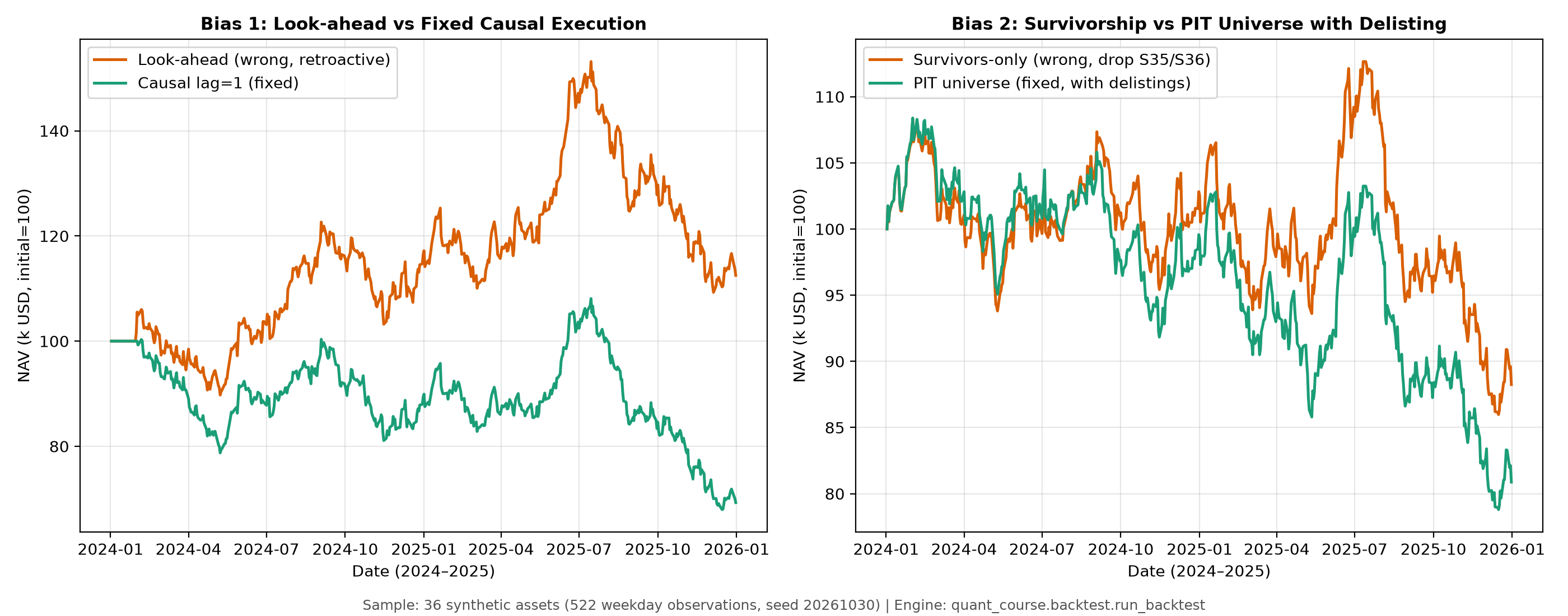
Left panel (Panel A: Look-ahead bias):
- Horizontal axis: synthetic Monday-to-Friday date grid (2024–2025; 522 observations, including exchange holidays); vertical axis: NAV (thousands of USD, initial value = 100).
- Comparison: the orange solid line is the look-ahead strategy (Wrong, retroactive), with ending NAV of 112500.12 USD and Sharpe of 0.3730; the green solid line is the causal strategy (decision at the close of the observation day after the announcement, then execution after lag=1), with ending NAV of 69300.37 USD and Sharpe of -0.7760.
- Main finding: the look-ahead strategy backdates after-hours announcement information to a signal before the announcement and establishes a position before the announcement gap. The causal strategy waits until a signal can be formed at the close and then executes.
Right panel (Panel B: Survivorship bias):
- Horizontal axis: the same 522-observation synthetic weekday grid; vertical axis: NAV (thousands of USD).
- Comparison: the orange solid line is the survivors-only strategy (Wrong, survivors-only), with ending NAV of 88.25 k USD and Sharpe of -0.2950; the green solid line is the true point-in-time strategy with delistings (Fixed, with delistings), with ending NAV of 80.87 k USD and Sharpe of -0.5565.
- Main finding: the universe containing only surviving stocks erases the two steep declines of S35 and S36 and creates a false impression of resilience.

10.2 Figure 2: Data-snooping multiple comparisons and selection bias

Data-snooping multiple comparisons and selection bias

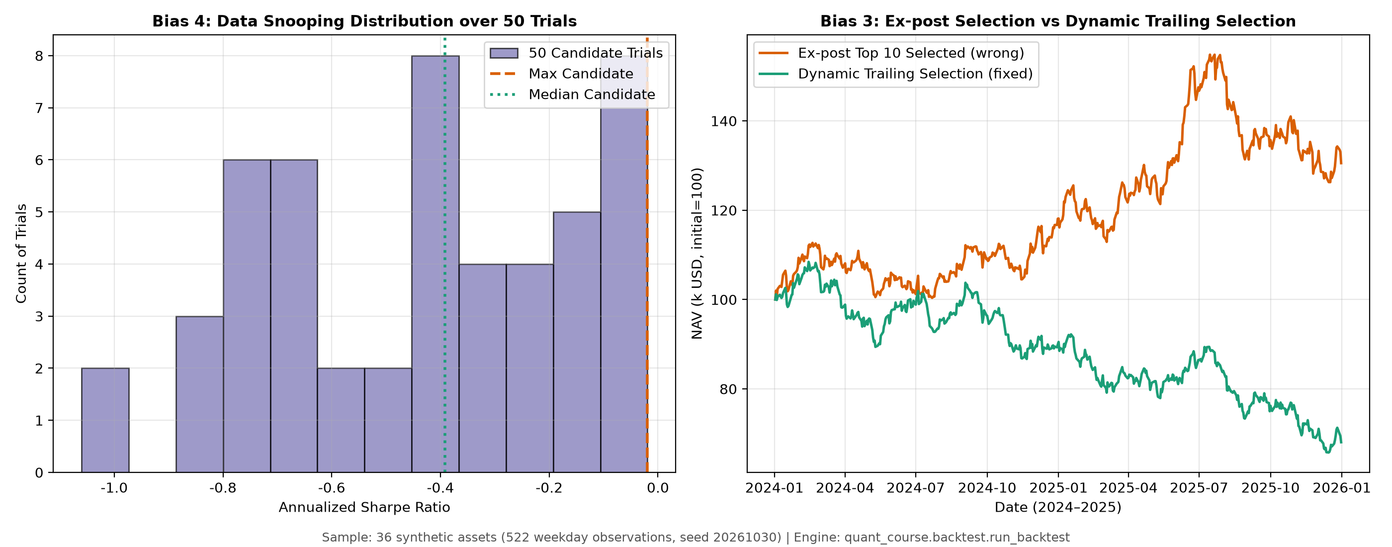
Left panel (Panel A: Data-snooping distribution):
- Horizontal axis: annualized Sharpe ratio; vertical axis: frequency of trials.
- Main finding: among 50 momentum strategies with different lookback periods, the median Sharpe is -0.3921 and even the maximum is -0.0193. Under the null, the expected maximum of 50 independent standard-normal trials is 2.2763 (BLdP approximation) and 2.2491 (exact value); the Bonferroni-adjusted p-value in this example is 1.0000. The candidate strategies are correlated and their returns do not satisfy the independent-normal assumption, so this is a teaching example about multiple comparisons, not a formal significance test.
Right panel (Panel B: Selection bias):
- Horizontal axis: the same 522-observation synthetic weekday grid; vertical axis: NAV (thousands of USD).
- Comparison: the orange solid line is the 10 stocks with the best full-period performance selected ex post (Wrong, ex-post), with ending NAV of 130.54 k USD and Sharpe of 0.8164; the green solid line is a dynamic screen based on a rolling 60-day economic-return Sharpe (Fixed, trailing 60d), with ending NAV of 68.06 k USD and Sharpe of -0.9108.

10.3 Figure 3: Overfitting decay and parameter-mining grid surface

Overfitting decay and parameter-mining grid surface

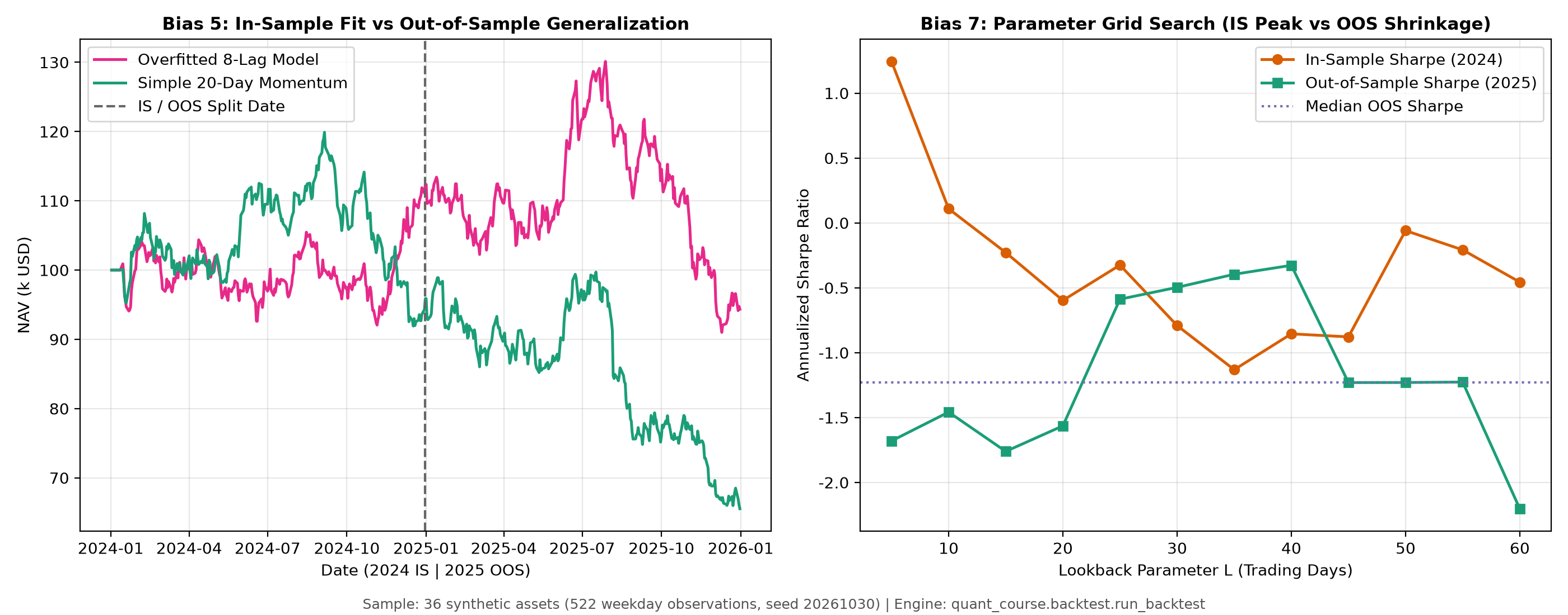
Left panel (Panel A: In-sample and out-of-sample overfitting comparison):
- Horizontal axis: date, with 2024-12-31 as the IS/OOS split; vertical axis: NAV.
- Main finding: the model uses eight close-to-close economic returns available through the signal close to predict the next trading day's gross open-to-close return. The unregularized regression (magenta) has IS Sharpe of 0.7041, falling to -0.6788 OOS; the 20-day momentum benchmark (green) has IS Sharpe of -0.1243 and OOS Sharpe of -1.5639. Neither shows stable OOS performance, and a single split cannot establish that the simple strategy is superior.
Right panel (Panel B: Parameter-mining grid):
- Horizontal axis: lookback parameter $L$ (5 to 60 days); vertical axis: annualized Sharpe ratio.
- Main finding: the parameter selected in the training period, $L^* = 5$ days, has IS Sharpe of 1.2443 and 2025 OOS Sharpe of -1.6799, a shrinkage of 2.9242. The selected parameter's OOS performance is below the median OOS value across the full grid, -1.2301; the grid's OOS results are for diagnosis only and do not enter parameter selection.

10.4 Figure 4: Corporate-action accounting and transaction-cost sensitivity

Corporate-action accounting and transaction-cost sensitivity

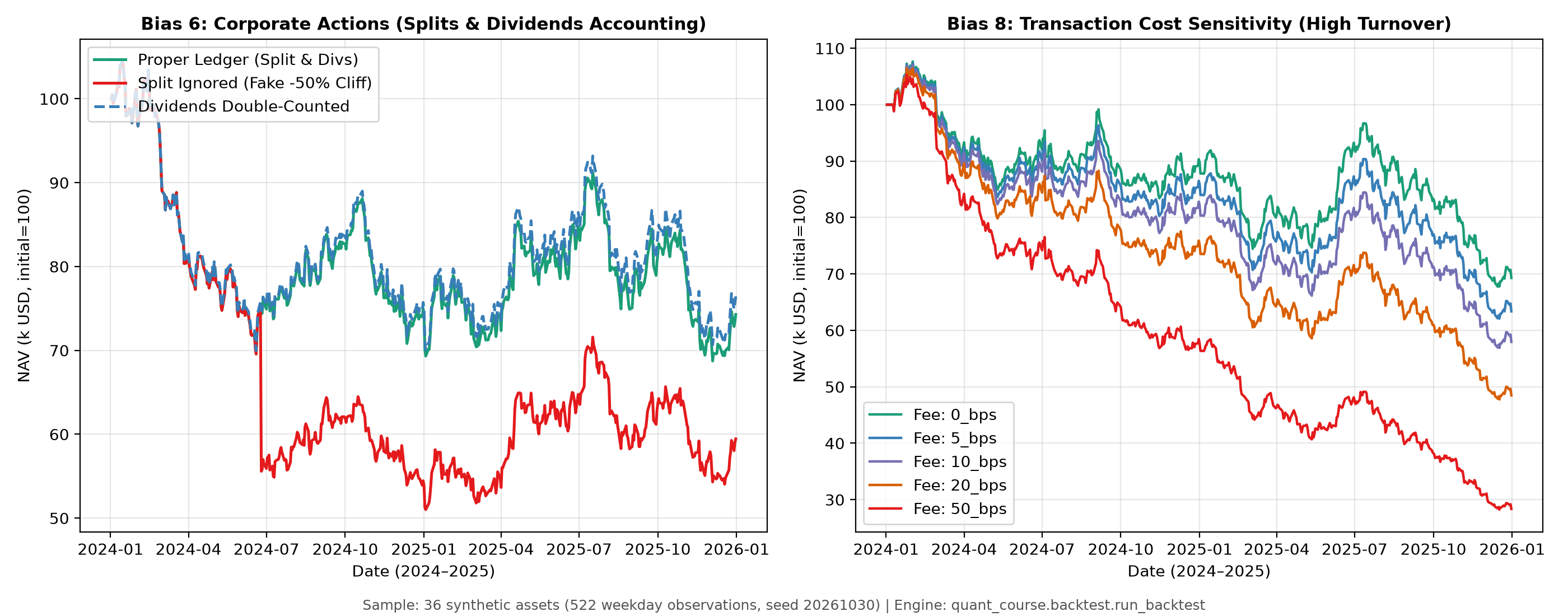
Left panel (Panel A: Corporate-action accounting):
- Main finding: the original figure's “Fake -50% Cliff” refers to the mechanical halving of one stock's market value when its shares are not adjusted; it is not the NAV decline of this portfolio. The historical sample for this portfolio shows -26.20%, while the cash/B mini-example in Section 3 shows -25%. The red line that ignores the split drops 26.20% on day 125 and ends at NAV of 59.45 k USD; the correctly reconciled green line transitions smoothly and ends at NAV of 74.28 k USD; the blue dashed line shows the artificial inflation from double-crediting dividends while using adjusted prices (ending NAV 76.44 k USD).
Right panel (Panel B: Transaction-cost ladder):
- Horizontal axis: the same 522-observation synthetic weekday grid; vertical axis: NAV.
- Main finding: in the high-turnover momentum strategy (annualized turnover of 6912.25% in the 10 bps scenario), ending NAV is 69.29 k USD (CAGR -16.23%) with a 0 bps one-way fee, 57.96 k USD (CAGR -23.15%) with a 10 bps fee, and 28.36 k USD (CAGR -45.58%) with a 50 bps fee. NAV and Sharpe both decline strictly as the fee rate rises.

11. Real Market Example

11.1 Historical-method example and its data-rights boundary

This section retains the historical methodological illustration previously based on Kenneth R. French's data. The raw, extracted, and processed data are not included in the default I3 package, and the rights, subjects, and intended uses remain unresolved. The A10-A design and A10-A.1 technical protocol do not replace execution authorization; G05/A10-B has not been authorized. The historical study is not rerun here. The previously used monthly returns for 10 industry portfolios illustrate selection bias over a long span of real historical data:

Data-source URL: https://mba.tuck.dartmouth.edu/pages/faculty/ken.french/ftp/10_Industry_Portfolios_CSV.zip
Industry-data manifest: data/manifests/french_industries_2026-10-05.json (SHA-256: 3b71cd5f781f9790cc380195c22635e03e9c9e27a5f43cd2d0d46fb12efa8271)
Raw industry ZIP SHA-256: ebd937a4b995d821867aeb956a96f09a666386f38fa82516b7d1767ee4a49ae5 (hash of the raw archive; it differs from the hash of the JSON manifest below)
Processed industry file: data/processed/french_10_industries_monthly.csv (SHA-256: 3b097d810c295d64eedfa1ece7067ff2a0707f5ca90e33935df9949251f70950)
Risk-free-rate manifest: data/manifests/french_factors_2026-10-05.json (SHA-256: 597c9703afa623a63b0d5fbf36dc941aac90d00948aeca302f151ed3c854000b)
Processed risk-free-rate file: data/processed/french_factors_3_monthly.csv (SHA-256: c19770a19a0ac47ad1c29074f57234570aeaa9725212cb4fa8146a2846c52814)
Sample period and frequency: 1926-07 through 2026-08, 1,202 consecutive monthly observations, with returns in decimal form per period.
Disclaimer and non-PIT status: Kenneth French's 10 industry data are aggregate, value-weighted industry portfolios for the full market. The historical data have been recalculated after multiple revisions; they are a non-point-in-time (non-PIT) snapshot and do not contain directly tradable, unadjusted constituent-stock quotes. This example cannot support a claim of live-trading alpha and is only a methodological illustration for academic research.

11.2 Fifty-year split: ex-post selection versus ex-ante selection

We compare two non-overlapping historical periods without assuming that the return series are statistically independent (figures are quoted from ch30_results.json["real_market_french"]):

Period 1 (1926-07 through 1975-12; 594 months): Sharpe ratios for the 10 industries are calculated over Period 1. The three highest-ranked industries are:
1. Hlth (Health): Sharpe = 0.4657
2. Telcm (Telecom): Sharpe = 0.4116
3. HiTec (High Tech): Sharpe = 0.4106
The equal-weighted portfolio of the top three industries in Period 1 has a Sharpe of 0.4701, compared with 0.4250 for the unconditional equal-weighted benchmark across all 10 industries; its excess Sharpe is +0.0451.
Full-sample view (1926-07 through 2026-08; 1,202 months): In the ex-post full-sample calculation, the top three industries by full-period Sharpe change to NoDur (0.5099), Hlth (0.5044), and Shops (0.4577).
Period 2 evaluation (1976-01 through 2026-08; 608 months): We compare the actual performance of three strategies in Period 2:
1. Wrong version (top three selected ex post using the full sample, with look-ahead selection bias): Holding the ex-post full-sample picks NoDur, Hlth, and Shops produces a Period 2 Sharpe of 0.6519 (CAGR = 13.15%), with excess Sharpe of +0.0372 relative to the equal-weighted 10-industry benchmark.
2. Fixed version (top three selected ex ante using Period 1 only): Holding only the Period 1 picks (Hlth, Telcm, and HiTec) in Period 2 produces an actual Sharpe of 0.5658 (CAGR = 12.46%), with excess Sharpe of -0.0489 relative to the equal-weighted 10-industry benchmark.
3. Benchmark portfolio (unconditional equal weight across 10 industries): The Period 2 Sharpe is 0.6147 (CAGR = 12.75%).

Metric definition and decay:

Sharpe difference between the wrong and fixed versions: 0.6519 - 0.5658 = +0.0862 (inflated by ex-post selection).
Change in the ex-ante portfolio's excess Sharpe (Excess Decay): its excess Sharpe relative to the benchmark changes from +0.0451 in Period 1 to -0.0489 in Period 2; the decline in excess Sharpe relative to the benchmark is:

$\text{Excess Decay} = (-0.0489) - (+0.0451) = -0.0940$

This value shows that the fixed portfolio selected using the first half of the sample did not maintain its excess Sharpe advantage over the benchmark in the second half.

12. Common Mistakes

This section examines eight forms of bias in depth. Each follows the same structure: “incorrect example → why it is wrong → runnable incorrect code → corrected code → numerical difference on the same data → limitations that remain after the correction.”

12.1 Bias 1: Look-ahead bias

Incorrect example: In a monthly-rebalanced model, a company releases a positive earnings preannouncement after the close at 16:30 on Friday, 2024-03-29. The researcher labels the announcement as a March feature and generates a trade instruction before the close on March 29, or even executes it that day.
Why it is wrong: The information release time $t_{\text{avail}} > s$ (Friday's close), so the information is not yet available at the Friday decision and execution times.
Runnable incorrect code (shows the timestamp being backdated):

import pandas as pd
from quant_course.backtest import BacktestConfig, run_backtest

dates = pd.bdate_range("2024-01-02", periods=3)
P = pd.DataFrame({"A": [10.0, 11.0, 12.0]}, index=dates)
E = pd.DataFrame({"A": [10.0, 11.0, 12.0]}, index=dates)
# Incorrect: the announcement occurs after the close on date 1 (16:30), but the signal is backdated to date 0.
# With lag=1, entry is early at 11 on date 1; this position does not earn the preceding 10-to-11 gap.
announcement_date = dates[1]
leaked_signal_date = dates[0]
tw_wrong = pd.DataFrame({"A": [1.0]}, index=[leaked_signal_date])
cfg = BacktestConfig(initial_cash=1000.0, lag=1)
res_wrong = run_backtest(P, tw_wrong, cfg, exec_prices=E)
assert res_wrong.fills["trade_time"].iloc[0] == dates[1]

This three-row example demonstrates backdating and invalid early entry only. The account buys at 11 on date 1 and is marked at 11 at that close, so its closing NAV remains USD 1,000; it does not earn the preceding 10-to-11 gap. The holding-period construction across the announcement in §6.1 and the historical results below use their own data and protocols; they are not outputs of this three-row code.

Corrected code (the announcement is released at 16:30 after the close on dates[1]; under a close-decision convention, the signal is formed at the next day's close on dates[2], and lag=1 executes at the open on dates[3]):

import pandas as pd
from quant_course.backtest import BacktestConfig, run_backtest

dates = pd.bdate_range("2024-01-02", periods=4)
P = pd.DataFrame({"A": [10.0, 11.0, 11.0, 11.0]}, index=dates)
E = pd.DataFrame({"A": [10.0, 11.0, 11.0, 11.0]}, index=dates)
# The 16:30 announcement on date[1] is unavailable at its close.
announcement_date = dates[1]
causal_signal_date = dates[2]
tw_fixed = pd.DataFrame({"A": [1.0]}, index=[causal_signal_date])
cfg = BacktestConfig(initial_cash=1000.0, lag=1)
res_fixed = run_backtest(P, tw_fixed, cfg, exec_prices=E)
assert res_fixed.fills["signal_time"].iloc[0] == dates[2]
assert res_fixed.fills["trade_time"].iloc[0] == dates[3]

Numerical difference on the same data (quoted from ch30_results.json["bias_1_lookahead"]):
- fixed (decision at the close of the observation day after the announcement): ending NAV = 69300.37 USD, Sharpe = -0.7760.
- wrong (future announcement backdated to a signal before its release): ending NAV = 112500.12 USD, Sharpe = 0.3730.
- Difference: NAV difference +43199.74 USD; Sharpe difference +1.1490 (sign: wrong > fixed).
Empirical distribution across 20 additional random seeds (quoted from ch30_results.json["multi_seed_distribution"]["lookahead_diff_sharpe"]):
- Mean difference: +1.1100; standard deviation: 0.2150; range: [0.7854, 1.6389]; positive-difference share: 100.0%. The main-seed difference, 1.1490, lies within the observed range across these 20 draws.
Limitations that remain after the correction: lag=1 means only that a signal executes at least on the next observation; by itself, it does not prove that an after-hours announcement was ingested before the order cutoff. This chapter's default uses after-hours announcements in a signal formed at the next observation day's close. An earlier decision requires the actual announcement time, receipt/ingestion time, and order cutoff time, with their ordering demonstrated. Causal timestamps still do not resolve one-price limit-up conditions, trading suspensions, execution capacity, or later restatements.

12.2 Bias 2: Survivorship bias

Incorrect example: Export “currently listed stocks” from a market-data application and use that list as the backtest universe for several preceding years.
Why it is wrong: The current list is a survivor set selected by past outcomes and automatically excludes failed companies that defaulted, were delisted, or were removed from the exchange.
Runnable incorrect code (builds the universe using future survival status):

import pandas as pd
from quant_course.backtest import BacktestConfig, run_backtest

dates = pd.bdate_range("2024-01-02", periods=4)
# Incorrect: at the start of the backtest (t=0), use end-of-period survival status to remove stock C, which is delisted on date 2.
all_universe = ["A", "B", "C"]
future_delisted = ["C"]
survivors_only = [s for s in all_universe if s not in future_delisted]
P_surv = pd.DataFrame({"A": [10.0, 11.0, 12.0, 13.0], "B": [20.0, 21.0, 22.0, 23.0]}, index=dates)
tw_wrong = pd.DataFrame({"A": [0.5], "B": [0.5]}, index=[dates[0]])
cfg = BacktestConfig(initial_cash=1000.0, lag=1)
res_wrong = run_backtest(P_surv, tw_wrong, cfg)
assert "C" not in res_wrong.positions.columns

Corrected code (uses the point-in-time full universe and records delisting):

import pandas as pd
from quant_course.backtest import BacktestConfig, run_backtest

dates = pd.bdate_range("2024-01-02", periods=4)
# Correction: retain the full universe that existed at the time; the delistings mapping liquidates the position for cash on the delisting date.
P_all = pd.DataFrame({
    "A": [10.0, 11.0, 12.0, 13.0],
    "B": [20.0, 21.0, 22.0, 23.0],
    "C": [10.0, 5.0, float("nan"), float("nan")]
}, index=dates)
tw_fixed = pd.DataFrame({"A": [0.33], "B": [0.33], "C": [0.34]}, index=[dates[0]])
cfg = BacktestConfig(initial_cash=1000.0, lag=1)
res_fixed = run_backtest(P_all, tw_fixed, cfg, delistings={"C": (dates[2], 1.0)})
assert res_fixed.ledger["delist_cash"].iloc[2] > 0

Numerical difference on the same data (quoted from ch30_results.json["bias_2_survivorship"]):
- fixed (PIT universe with delisting liquidation): ending NAV = 80874.56 USD, Sharpe = -0.5565.
- wrong (survivors only): ending NAV = 88245.23 USD, Sharpe = -0.2950.
- Difference: NAV difference +7370.67 USD; Sharpe difference +0.2616 (sign: wrong > fixed).
Empirical distribution across 20 additional random seeds (quoted from ch30_results.json["multi_seed_distribution"]["survivorship_diff_sharpe"]):
- Mean difference: +0.3174; standard deviation: 0.0306; range: [0.2677, 0.3894]; positive-difference share: 100.0%. The main-seed difference of 0.2616 and the 20 positive differences are retained as observations from their respective constructed draws; they do not establish a robust direction across all markets or seeds.
Limitations that remain after the correction: A PIT universe and recorded delisting liquidation still do not resolve off-exchange transfer slippage at a discount during a delisting suspension, or the omission of micro-cap delisted stocks from early vintages of a historical full-universe database.

12.3 Bias 3: Selection bias

Incorrect example: Inspect the full-sample results for the stock universe over 2024–2025, then put the best-performing stocks into the backtest portfolio in advance.
Why it is wrong: The selection rule is conditional on future full-sample outcomes.
Runnable incorrect code (selects stocks using a full-sample ex-post metric):

import pandas as pd
from quant_course.backtest import BacktestConfig, run_backtest

dates = pd.bdate_range("2024-01-02", periods=4)
P = pd.DataFrame({"A": [10.0, 15.0, 18.0, 20.0], "B": [20.0, 18.0, 16.0, 15.0]}, index=dates)
# Incorrect: after the full sample ends, select stocks using their mean return over all dates; this small example has no corporate actions.
full_sample_top = P.pct_change().dropna().mean().idxmax()
assert full_sample_top == "A"
tw_wrong = pd.DataFrame({full_sample_top: [1.0]}, index=[dates[0]])
cfg = BacktestConfig(initial_cash=1000.0, lag=1)
res_wrong = run_backtest(P[[full_sample_top]], tw_wrong, cfg)
assert res_wrong.ledger["nav"].iloc[-1] > 1000.0

Corrected code (dynamic ex-ante selection using only a historical rolling window):

import pandas as pd
from quant_course.backtest import BacktestConfig, run_backtest

dates = pd.bdate_range("2024-01-02", periods=6)
P = pd.DataFrame({"A": [10.0, 11.0, 10.0, 12.0, 11.0, 13.0],
                  "B": [10.0, 9.0, 10.0, 9.0, 11.0, 10.0]}, index=dates)
# This small example has no corporate actions. At each close decision, compare only the preceding two days of returns.
daily_returns = P.pct_change()
rows = []
for i in range(2, len(dates) - 1):
    trailing_mean = daily_returns.iloc[i - 1:i + 1].mean()
    selected = trailing_mean.idxmax()
    rows.append({"A": float(selected == "A"), "B": float(selected == "B")})
tw_fixed = pd.DataFrame(rows, index=dates[2:-1])
cfg = BacktestConfig(initial_cash=1000.0, lag=1)
res_fixed = run_backtest(P, tw_fixed, cfg)
assert tw_fixed.nunique().iloc[0] > 1 or tw_fixed.nunique().iloc[1] > 1
assert res_fixed.ledger["nav"].iloc[-1] > 0

Numerical difference on the same data (quoted from ch30_results.json["bias_3_selection"]; this comparison uses the full PIT universe that includes delisted S35 and S36):
- fixed (rolling dynamic forward selection): ending NAV = 68057.83 USD, Sharpe = -0.9108.
- wrong (10 best stocks selected ex post): ending NAV = 130536.57 USD, Sharpe = 0.8164.
- Difference: NAV difference +62478.74 USD; Sharpe difference +1.7272 (sign: wrong > fixed).
Empirical distribution across 20 additional random seeds (quoted from ch30_results.json["multi_seed_distribution"]["selection_diff_sharpe"]):
- Mean difference: +1.2671; standard deviation: 0.3014; range: [0.6812, 1.8841]; positive-difference share: 100.0%.
Limitations that remain after the correction: A dynamic ex-ante rule still needs a declared target population. If a “continuously profitable in the past” condition was known at the time, it can define a legitimate prespecified investment universe. The corresponding selection problem arises only when this conditional population is presented as an unconditional result for the whole market or future eligibility is written back into the historical record.

12.4 Bias 4: Data snooping

Incorrect example: Try 50 momentum signals with different lookback periods on the same historical dataset, report only the one with the highest backtest Sharpe, and claim to have found significant alpha.
Why it is wrong: Taking the maximum of independent random variables systematically inflates the nominal test statistic and ignores extreme-value inflation under multiple testing.
Runnable incorrect code (reports only the maximum without logging the multiple trials):

import numpy as np

# Fifty candidate return series on a fixed sample; the incorrect approach reports only the best Sharpe.
rng = np.random.default_rng(30)
trial_returns = rng.normal(0.0002, 0.01, size=(522, 50))
sharpes = trial_returns.mean(axis=0) / trial_returns.std(axis=0, ddof=1) * np.sqrt(252)
best_metric = float(sharpes.max())
assert np.isfinite(best_metric)

Corrected code (logs every trial in TrialLedger and adjusts the full p-value vector with Bonferroni):

import numpy as np
from scipy import stats
from quant_course.research_protocol import TrialLedger, bonferroni_adjust

# Retain all 50 candidate return series from the incorrect example and record every trial.
rng = np.random.default_rng(30)
trial_returns = rng.normal(0.0002, 0.01, size=(522, 50))
ledger = TrialLedger()
p_values = []
for m, daily_returns in enumerate(trial_returns.T):
    sharpe = float(daily_returns.mean() / daily_returns.std(ddof=1) * np.sqrt(252))
    t_stat = sharpe * np.sqrt(len(daily_returns) / 252)
    p_values.append(float(2 * stats.norm.sf(abs(t_stat))))
    ledger.record({"candidate": m + 1}, metric=sharpe, n_obs=len(daily_returns))

assert ledger.n_trials == 50
p_bonf_all = bonferroni_adjust(np.array(p_values))
# Pass the full vector of 50 p-values to apply the multiple-comparison adjustment automatically.
assert (p_bonf_all >= np.array(p_values)).all()

Numerical difference on the same data (quoted from ch30_results.json["bias_4_data_snooping"]):
- Number of candidate trials: 50.
- Maximum selected Sharpe: -0.0193 (median: -0.3921; mean: -0.4369).
- Expected maximum across 50 normal trials under the null: exact value = 2.2491; BLdP approximation = 2.2763; Gumbel approximation = 2.3072.
- Nominal p-value = 0.9782; Bonferroni-adjusted p-value = 1.0000.
Limitations that remain after the correction: A trial ledger can constrain attempts made by mechanical code, but it cannot resolve informal trials left unrecorded in a researcher's mind (Mental Trials) or the data snooping produced by decades of collective trial and error on public data in academia.

12.5 Bias 5: Overfitting

Incorrect example: In 2024 (the in-sample, IS period), fit the next trading day's return using eight historical-return features, then treat the in-sample fit as future performance.
Why it is wrong: The model has too many degrees of freedom, forcing it to memorize idiosyncratic in-sample noise without structural generalization.
Runnable incorrect code (fits a high-degree polynomial only in sample):

import numpy as np

# Incorrect: fit only on the training sample and leave no out-of-sample validation.
rng = np.random.default_rng(2)
x = rng.uniform(-1, 1, 30)
y = 0.6 * x + rng.normal(0, 0.3, size=30)
x_is, y_is = x[:20], y[:20]
poly_overfit = np.polyfit(x_is, y_is, deg=8)
assert len(poly_overfit) == 9
# The target includes random noise; fit on training only is not out-of-sample evidence.

Corrected code (constrains the model and validates on a held-out sample):

import numpy as np

# Fix the random seed; split the training and held-out periods in time order, and fit using only the training segment.
rng = np.random.default_rng(2)
x = rng.uniform(-1, 1, 30)
y = 0.6 * x + rng.normal(0, 0.3, size=len(x))
split = 20
poly_overfit = np.polyfit(x[:split], y[:split], deg=8)
poly_simple = np.polyfit(x[:split], y[:split], deg=1)
train_mse_overfit = np.mean((y[:split] - np.polyval(poly_overfit, x[:split])) ** 2)
train_mse_simple = np.mean((y[:split] - np.polyval(poly_simple, x[:split])) ** 2)
test_mse_overfit = np.mean((y[split:] - np.polyval(poly_overfit, x[split:])) ** 2)
test_mse_simple = np.mean((y[split:] - np.polyval(poly_simple, x[split:])) ** 2)
assert train_mse_overfit < train_mse_simple
assert test_mse_overfit > test_mse_simple

In this fixed random example, the degree-8 model's training MSE is about 0.0382 and its held-out MSE is about 0.2412. A single holdout can assess generalization over that period, but cannot establish future stability.
The strategy-level label in the constructed-market CLI is strictly the gross open-to-close return on the trading day after the signal-day close; the eight features are economic close-to-close returns available through the signal close. The overnight gap occurs before execution and is not included in the new position's label. Backtest NAV is still calculated from raw prices, corporate actions, and the fee ledger.
Numerical difference on the same data (quoted from ch30_results.json["bias_5_overfitting"]):
- Eight-feature regression: IS Sharpe = 0.7041; OOS Sharpe = -0.6788; change = -1.3829.
- 20-day momentum benchmark: IS Sharpe = -0.1243; OOS Sharpe = -1.5639; change = -1.4396. Neither strategy generalized in this constructed sample, so this does not support a claim that the simple benchmark is superior.
Limitations that remain after the correction: A simple out-of-sample split can reveal overfitting, but cannot resolve iterative leakage from repeatedly inspecting OOS results and then changing the model. Chapter 31 formalizes this issue further with Purged CV and Embargo.

12.6 Bias 6: Incorrect corporate-action handling

Incorrect examples:
- Error A: use unadjusted prices directly in the backtest without passing a splits table to the engine.
- Error B: backtest using adjusted prices while also enabling cash credits through a dividends table.
Why they are wrong:
- Error A halves the share price on the ex-split date without doubling the share count, creating an artificial 50% crash.
- Error B credits dividends a second time in the cash ledger even though the adjusted prices already reflect dividend reinvestment, double-counting the dividend return.
Runnable incorrect code (shows the artificial drop caused by omitting the split parameter):

import pandas as pd
from quant_course.backtest import BacktestConfig, run_backtest

dates = pd.bdate_range("2024-01-02", periods=4)
# Incorrect: S05 undergoes a 2:1 split, but the splits parameter is omitted, causing an artificial crash.
P = pd.DataFrame({"S05": [100.0, 100.0, 50.0, 50.0]}, index=dates)
tw = pd.DataFrame({"S05": [1.0, 1.0, 1.0, 1.0]}, index=dates)
cfg = BacktestConfig(initial_cash=1000.0, lag=1)
res_wrong = run_backtest(P, tw, cfg)
# On day 2 the position is held through the split, but the share count is not adjusted; NAV drops 50%.
assert res_wrong.ledger["nav"].iloc[2] == 500.0

Corrected code (passes raw prices and a split-multiplier table):

import pandas as pd
from quant_course.backtest import BacktestConfig, run_backtest, reconcile

dates = pd.bdate_range("2024-01-02", periods=4)
# Correction: pass unadjusted prices and the split-multiplier table.
P = pd.DataFrame({"S05": [100.0, 100.0, 50.0, 50.0]}, index=dates)
splits = pd.DataFrame({"S05": [1.0, 1.0, 2.0, 1.0]}, index=dates)
tw = pd.DataFrame({"S05": [1.0, 1.0, 1.0, 1.0]}, index=dates)
cfg = BacktestConfig(initial_cash=1000.0, lag=1)
res_fixed = run_backtest(P, tw, cfg, splits=splits)
rec = reconcile(res_fixed, P, cfg, splits=splits)
assert rec["residual"].abs().max() < 1e-12

Error B and its correction: double-crediting a dividend when using adjusted prices. The flat adjusted-price series below already incorporates the total return from a USD 1 dividend. Passing a dividends table to the ledger as well adds another USD 10. Production backtests should use unadjusted execution/mark prices with a clearly identified source, and pass corporate actions separately:

import pandas as pd
from quant_course.backtest import BacktestConfig, run_backtest

dates = pd.bdate_range("2024-01-02", periods=4)
tw = pd.DataFrame({"A": [1.0]}, index=[dates[0]])
dividends = pd.DataFrame({"A": [0.0, 0.0, 1.0, 0.0]}, index=dates)
cfg = BacktestConfig(initial_cash=1000.0, lag=1)

# Wrong: adjusted close is flat, while the ledger also credits a 1 USD dividend.
P_adjusted = pd.DataFrame({"A": [100.0, 100.0, 100.0, 100.0]}, index=dates)
wrong = run_backtest(P_adjusted, tw, cfg, dividends=dividends)

# Fix: use raw prices; record the 100-to-99 ex-date move and the 1 USD/share cash.
P_raw = pd.DataFrame({"A": [100.0, 100.0, 99.0, 99.0]}, index=dates)
fixed = run_backtest(P_raw, tw, cfg, dividends=dividends)
assert fixed.ledger["nav"].iloc[2] == 1000.0
assert wrong.ledger["nav"].iloc[2] == 1010.0

Numerical difference on the same data (quoted from ch30_results.json["bias_6_corporate_actions"]):
- fixed (compliant unadjusted-price accounting): ending NAV = 74281.57 USD; return on the split date = -0.0129.
- split_ignored: ending NAV = 59445.09 USD; return on the split date = -0.2620 (an artificial 26.20% drop).
- dividend_double_counted: ending NAV = 76444.05 USD (an overstatement of USD 2,162.48).
- Maximum absolute ledger-reconciliation residual: 2.55e-11 USD (an internal accounting check at the stated scale; it does not prove that market-price inputs or all trading conditions are correct).
Limitations that remain after the correction: Correctly entering splits and dividends can maintain cash-and-share accounting, but does not resolve complex subsidiary spin-offs, rights-offering dilution discounts, or differences in dividend withholding taxes across international markets.

12.7 Bias 7: Parameter mining

Incorrect example: Run a dense in-sample grid search over momentum lookback days $L \in \{5, 10, \dots, 60\}$ and choose the in-sample optimum, $L^* = 5$ days, as the live-trading parameter.
Why it is wrong: It treats a local maximum from a discrete sample as a deep market invariant and ignores the parameter surface's flatness and the risk of overfitting.
Runnable incorrect code:

import importlib.util
from pathlib import Path

spec = importlib.util.spec_from_file_location("ch30", Path("code/ch30_backtest_biases.py"))
ch30 = importlib.util.module_from_spec(spec)
spec.loader.exec_module(ch30)
data = ch30.build_constructed_market(seed=20261030)
# The parameter-scan function returns the actual in-sample performance of the backtest.
result = ch30.study_parameter_mining(data)
grid = result["grid"]
best_is = max(grid, key=lambda row: row["is_sharpe"])
# Incorrect interpretation: treat the in-sample peak as a future-realizable Sharpe.
claimed_future_sharpe = best_is["is_sharpe"]
assert best_is["lookback"] == result["best_is_lookback"]

Corrected code (selects parameters in the training period and evaluates the selected parameter only in the test period):

import importlib.util
from pathlib import Path

spec = importlib.util.spec_from_file_location("ch30", Path("code/ch30_backtest_biases.py"))
ch30 = importlib.util.module_from_spec(spec)
spec.loader.exec_module(ch30)
data = ch30.build_constructed_market(seed=20261030)
result = ch30.study_parameter_mining(data)
best_L = result["best_is_lookback"]  # selected on the 2024 IS segment only
selected_oos_sharpe = result["best_param_oos_sharpe"]
print(f"Selected on 2024 only: L={best_L}; 2025 Sharpe={selected_oos_sharpe:.4f}")

Numerical difference on the same data (quoted from ch30_results.json["bias_7_parameter_mining"], after correcting the warm-up window):
- Best in-sample parameter: $L^* = 5$ days; in-sample Sharpe = 1.2443.
- Actual out-of-sample performance for that parameter: OOS Sharpe = -1.6799.
- Median OOS value across the full grid: -1.2301.
- OOS shrinkage: 2.9242 (from a positive mean return to the negative-return region).
Empirical distribution across 20 additional random seeds (quoted from ch30_results.json["multi_seed_distribution"]["parameter_mining_oos_shrinkage"]):
- Mean OOS shrinkage: 0.3974; standard deviation: 1.4743; positive-shrinkage share: 55.0%. The shrinkage direction differs across random seeds, so the evidence does not support a universal effect.
Limitations that remain after the correction: Showing the full parameter surface reveals fragility, but does not resolve structural regime shifts that cause the true optimal parameter to drift over time.

12.8 Bias 8: Incorrect cost modeling

Incorrect example: Develop a high-turnover momentum strategy with fee_rate = 0.0 in the backtest and claim that its annualized return is robust.
Why it is wrong: It ignores market frictions. The proportional-fee illustration used consistently in this chapter has a material compounding effect on a high-turnover portfolio.
Runnable incorrect code:

import pandas as pd
from quant_course.backtest import BacktestConfig, run_backtest

dates = pd.bdate_range("2024-01-02", periods=3)
P = pd.DataFrame({"A": [10.0, 11.0, 12.0]}, index=dates)
cfg_zero = BacktestConfig(initial_cash=1000.0, fee_rate=0.0, lag=1)
res_zero = run_backtest(P, pd.DataFrame({"A": [1.0]}, index=[dates[0]]), cfg_zero)
assert res_zero.ledger["fees"].sum() == 0.0

Corrected code:

import pandas as pd
from quant_course.backtest import BacktestConfig, run_backtest

dates = pd.bdate_range("2024-01-02", periods=3)
P = pd.DataFrame({"A": [10.0, 11.0, 12.0]}, index=dates)
cfg_fee = BacktestConfig(initial_cash=1000.0, fee_rate=0.001, lag=1)
res_fee = run_backtest(P, pd.DataFrame({"A": [1.0]}, index=[dates[0]]), cfg_fee)
assert res_fee.ledger["fees"].sum() > 0.0

Numerical difference on the same data (quoted from ch30_results.json["bias_8_cost_modeling"]):
- Annualized turnover: 6912.25%.
- Fee rate of 0 bps: ending NAV = 69293.03 USD; CAGR = -16.23%; Sharpe = -0.7744; total fees = 0.0 USD.
- Fee rate of 5 bps: ending NAV = 63373.14 USD; CAGR = -19.76%; Sharpe = -0.9870; total fees = 7465.42 USD.
- Fee rate of 10 bps: ending NAV = 57958.45 USD; CAGR = -23.15%; Sharpe = -1.1984; total fees = 14318.22 USD.
- Fee rate of 20 bps: ending NAV = 48476.06 USD; CAGR = -29.50%; Sharpe = -1.6158; total fees = 26386.78 USD.
- Fee rate of 50 bps: ending NAV = 28356.82 USD; CAGR = -45.58%; Sharpe = -2.7949; total fees = 52420.09 USD.

The metrics decline strictly as the fee rate rises.

Limitations that remain after the correction: The proportional-fee model covers linear commissions and regulatory fees, but does not resolve nonlinear market impact for large orders (such as the square-root law), stock-borrow costs and short-sale constraints, or liquidity droughts in extreme markets.

13. Quant Research Application

In professional institutional quantitative research, backtest-bias defenses cannot rely on researchers' diligence alone. They must be built into fully automated CI/CD gates:

[Researcher submits strategy code and configuration]
               |
               v
   [Gate 1: automated future-perturbation invariance check]
   (inject Gaussian noise after cutoff time t; assert historical signals/fills/nav
    before t remain exactly identical)
               | (pass)
               v
   [Gate 2: static scan of point-in-time (PIT) contracts]
   (check release/ingestion/decision channels; shift(-1) may validly construct
    labels, but its actual support must be checked when used for features)
               | (pass)
               v
   [Gate 3: TrialLedger audit]
   (extract the cumulative number of trials M; calculate Bonferroni/Holm
    thresholds and expected extreme-value inflation)
               | (pass)
               v
   [Gate 4: unadjusted-price, self-financing ledger execution and cost ladder]
   (bind actual shares to unadjusted prices/corporate actions; do not credit
    dividends again for a declared total-return proxy; check fees and reconciliation)
               | (pass)
               v
[Eligible to proceed to Chapter 31's out-of-sample splits and Chapter 32's inference process]

14. Chapter Summary

14.1 Bias-diagnostic checklist: “What information, when available, and where used?”

Before deploying any backtest, quantitative engineers should rigorously check each item in the following table:

Review dimension	Core checklist question	Red flags	Architectural solution
Information timing (Available When)	Was this field officially released by the exchange or data vendor by the backtest decision time $s$ ?	Using period_end or placing after-hours announcements directly into same-day features	Filter using both release and ingestion clocks, then check the decision time and delayed execution
Universe completeness (Which Universe)	Does the asset universe include all names that went bankrupt, were delisted, or were suspended during the backtest period?	Using the latest current-stock list; filtering symbols based on a special identifier	Maintain a dynamic PIT constituent database with delisting liquidation-price mappings
Selection objectivity (Used Where)	Was the choice of names or factors based on historical performance over the full sample?	“Allocate the portfolio to the stocks/industries with the best performance over the past three years”	Build the benchmark using only historical information available up to each cross-section date
Search multiplicity (How Many Tried)	How many variants did the code and algorithms try before the final strategy was chosen?	The paper or report omits the number of trials and reports only one attractive backtest	Require TrialLedger to record all attempts and calculate adjusted thresholds
Generalization	Does the number of free parameters match the effective number of independent observations?	Very high in-sample Sharpe followed by a rapid fall to negative returns out of sample	Strictly separate training and test sets, and introduce regularization and cross-validation gates
Accounting conservation	Do share count and cash accounting preserve value through splits and dividends?	Using adjusted prices as execution prices; NAV suddenly halves on the ex-date	Input only actual unadjusted prices and run the reconcile ledger
Parameter surface (Sensitivity)	Is the optimum an isolated peak? How does performance change under small parameter perturbations?	A small change in a 5-day parameter flips backtest Sharpe from positive to negative	Scan the full parameter-sensitivity surface and evaluate shrinkage toward the median
Realism of frictions (Friction Reality)	How does the strategy perform under explicit proportional-fee, slippage, and stock-borrow assumptions?	Assuming zero commissions; high-turnover strategy is highly sensitive to the fee rate	Run the 0/5/10/20/50 bps ladder and calculate the turnover threshold

15. Exercises

30-E01 (Conceptual: point-in-time causal inequality): On a discrete trading timeline, let the signal decision time be the close at $s$ , and let the order execution time be $t_{\text{trade}} = s + \text{lag}$ . If a macroeconomic data release occurs at 16:30 on date $s$ , write the point-in-time causal inequality that constrains when the strategy may use that data. Explain separately whether ingestion at 09:45 on the next day prevents a decision at that day's close, and why it would violate a different premarket-decision contract that requires the order to be placed before 09:30 the next day. Do not conflate the two clocks.
30-E02 (Mathematical: survivorship-bias premium under a truncated normal distribution): Suppose the one-period stock return is $R \sim \mathcal{N}(0.01, 0.04^2)$ . If a strategy counts only surviving names whose return is at least $-0.03$ , use numerical values of the standard-normal density $\phi$ and cumulative distribution function $\Phi$ to calculate by hand the conditional mean return $\mathbb{E}[R \mid R \ge -0.03]$ for the surviving sample. Then calculate the one-period upward bias in the mean and the difference in the annualized arithmetic mean after multiplying by 252. Explain why the latter is not an achievable compounded annual return.
30-E03 (Mathematical: expected maximum-Sharpe inflation under multiple testing): Under the null hypothesis (true Sharpe ratio equal to 0), a quantitative team independently evaluates $M = 100$ factors. Use the extreme-value expectation approximation

$\mathbb{E}[M_M] \approx \sqrt{2\ln M} - \frac{\ln\ln M + \ln(4\pi)}{2\sqrt{2\ln M}} + \frac{\gamma}{\sqrt{2\ln M}}$
to calculate by hand the expected test statistic for the best factor. Then use the null distribution of the maximum, or an effective multiplicity-adjusted p-value, to determine whether a one-sided nominal statistic of 2.0 is significant at a 5% family-wise level. Do not compare it only with the expected maximum.
30-E04 (Proof: split neutrality in an unadjusted-price self-financing ledger): On date $t$ , suppose the number of shares changes from $q_{t-1}$ to $q_{t-1} \cdot S_t$ , while the closing price changes from $P_{t-1}$ to $P_{t-1} / S_t$ . Prove that on a pure ex-split date with no cash dividend and no rebalancing, the ledger's daily reconciliation residual $\text{residual}_t$ is identically 0 and the first derivative of total NAV with respect to the split ratio $S_t$ is 0 everywhere.
30-E05 (Derivation: transaction-cost breakeven for a high-turnover strategy): Define $\tau_{L1}=\sum_i |\Delta x_i|/V_{\text{pre}}$ as the total L1 turnover used by the ledger (buy notional plus sell notional), and let $c$ be the one-way proportional trading-fee rate. First define whether $r_g$ is the accounting return before fees on the same holdings, or the no-fee counterfactual return after fees are deducted before reinvestment. Write the end-of-period wealth-growth equation after transaction costs for each definition. Derive an approximate lower bound on the gross-return-to-turnover ratio $\frac{r_g}{\tau_{L1}}$ required for the strategy to achieve positive long-run compound growth ( $\mathbb{E}[\ln(1 + r_{\text{net}})] > 0$ ). If one-sided turnover is defined as $\tau_{1w}=\tau_{L1}/2$ , how does the cost coefficient in the equation change?

16. Programming Exercises

30-P01 (Future-perturbation non-intrusion checker): Write a general Python check function assert_future_perturbation_invariant that takes a strategy function, market data, and a cutoff date. Perturb raw mark prices, execution prices, announcements, splits, dividends, and future delisting-liquidation data after the cutoff, then rerun the strategy. Assert that target weights, fills, positions, and NAV through and including the cutoff date match the original results. The strategy interface should return (target_weights, BacktestResult).
30-P02 (Automatic multiple-testing adjustment using TrialLedger): Based on TrialLedger in src/quant_course/research_protocol.py, write an analysis function that takes a trial ledger and valid nominal p-values fully aligned by trial_id. Return the maximum and median metric, all nominal p-values, the Bonferroni and Holm adjusted sequences (in original candidate order and sorted order), and the rejected candidate IDs. Rejecting the null hypothesis does not establish that a strategy is “truly significant.”
30-P03 (Point-in-time dynamic constituent filter and delisting-liquidation allocator): Write a dynamic-weight function that takes mappings of listing and delisting dates and, on each monthly rebalance date, outputs a $1/N$ equal-weight target-weight matrix containing only the stocks still listed then. If a stock is delisted while held, close it at the given delisting liquidation price and return the cash to the cash ledger.
30-P04 (Double-counting detector for adjusted prices and an unadjusted ledger): Write a defensive validation module that requires callers to provide the price basis from source metadata (raw_unadjusted or adjusted). Allow prices to enter a ledger together with a cash-dividend table only when the basis is explicitly declared raw_unadjusted. An ex-dividend price drop may produce a diagnostic warning, but cannot by itself prove whether prices are adjusted; explain why the diagnostic can produce false positives and false negatives.

17. Challenge Problems

30-C01 (Open challenge: PIT causal isolation for restated financial statements): In real company financial statements, listed companies often publish restatements (10-K/A) several quarters or even years later, revising historical quarterly net income and equity. If a quantitative team wants to backtest a stock-selection strategy based on return on equity (ROE), design an underlying data architecture with a version table, an effective timestamp (pit_effective_at), and a dual-key alignment mechanism. Show why historical signal generation cannot be contaminated by future accounting restatements.
30-C02 (Open challenge: estimating effective independent trials in a continuous parameter search): In a moving-average crossover strategy, short-period parameter $S \in [5, 20]$ and long-period parameter $L \in [30, 120]$ are continuous or densely gridded, and the return series for neighboring grid points are highly correlated. Applying Bonferroni directly using the total number of grid points (for example, $15 \times 90 = 1350$ ) may be conservative. Propose an estimate based on eigenvalue decomposition of the return-correlation matrix or an effective number of tests ( $M_{\text{eff}}$ ), and give a counterexample showing when that estimate can fail.
30-C03 (Derivation challenge: feasibility of a closed-form solution for nonlinear market impact and a self-financing equation): Chapter 29 gives the post-fee NAV equation under proportional linear fees: $V' = V - c \sum_i |w_i V' - x_i|$ . Let $z_i=|\Delta x_i|=|w_i V'-x_i|$ , and consider total cost

$C_i(z_i)=c_1 z_i+c_2\sigma_i z_i\sqrt{z_i/\text{ADV}_i},$
where $z_i$ and $\text{ADV}_i$ are notionals in the same currency, $\sigma_i$ is a dimensionless return volatility, $c_1$ is a fee rate, and $c_2$ is dimensionless. Give sufficient conditions that guarantee a unique positive root on $[0,V_{\text{pre}}]$ , explain why Newton iteration is no longer presumed to converge monotonically, and describe how to use a bracketing root-finder if the conditions fail, including which conclusions can and cannot be drawn.

18. Solutions / Solution Hints

18.1 Full solutions to conceptual and derivation problems

30-E01 Solution

The release and ingestion clocks jointly determine the available time: $a(e)=\max(t_{\mathrm{avail}},t_{\mathrm{ingest}})$ . A valid feature requires $a(e)\le s_{\mathrm{close}}$ ; weights must be measurable with respect to $\mathcal F_s$ , and execution occurs at a later valid observation step.
Under the teaching clock in this problem, the market closes at 15:00 and the announcement arrives at 16:30, so it cannot be used for that day's close. If it has been ingested by 09:45 the next day, it can be used for that day's 15:00 close decision; after lag=1, execution occurs at the open of the following observation day. The 09:45 ingestion does not introduce look-ahead on this route.
If the contract instead forms a premarket order before 09:30 the next day, ingestion at 09:45 is after the decision and cutoff, so the data cannot be assumed available. The same lag label cannot replace checking the ordering of the actual release, ingestion, and order-cutoff times. If ingestion occurs later than the next close, the close-decision route in this problem must also be delayed.

30-E02 Solution

Standardized truncation point:

$\alpha = \frac{-0.03 - 0.01}{0.04} = \frac{-0.04}{0.04} = -1.0$
Tabulated values: The standard-normal density is $\phi(-1.0) = \frac{1}{\sqrt{2\pi}} e^{-0.5} \approx 0.24197$ . The cumulative distribution is $\Phi(-1.0) = 1 - \Phi(1.0) \approx 1 - 0.84134 = 0.15866$ .
Inverse Mills ratio:

$\lambda(-1.0) = \frac{\phi(-1.0)}{1 - \Phi(-1.0)} = \frac{0.24197}{0.84134} \approx 0.28760$
Conditional expectation:

$\mathbb{E}[R \mid R \ge -0.03] = 0.01 + 0.04 \times 0.28760 = 0.01 + 0.01150 = 0.02150 \quad (2.150\%)$
Spurious upward bias: The unrounded one-period mean difference is about 0.011504, or 1.1504 percentage points. Multiplying by 252 gives about 2.8990, or an annualized arithmetic-mean difference of 289.90 percentage points. This is a rescaling under the one-period truncation model; it is neither an achievable compounded annual return nor a conclusion under a condition that the same company survives to year-end.

30-E03 Solution

Calculate the logarithmic terms: Given $M = 100$ , $\ln 100 \approx 4.60517$ . $\sqrt{2\ln M} = \sqrt{2 \times 4.60517} = \sqrt{9.21034} \approx 3.03485$ . $\ln\ln 100 = \ln(4.60517) \approx 1.52723$ . $\ln(4\pi) = \ln(12.56637) \approx 2.53102$ .
Substitute into the formula for the expected maximum:

$\mathbb{E}[M_{100}] \approx 3.03485 - \frac{1.52723 + 2.53102}{2 \times 3.03485} + \frac{0.57722}{3.03485}$
$= 3.03485 - \frac{4.05825}{6.06970} + 0.19020 = 3.03485 - 0.66861 + 0.19020 \approx 2.55644$
Post-selection significance: The value 2.55644 is an asymptotic expectation approximation; it is not a 5% critical value. For the maximum of 100 independent one-sided standard-normal tests, at an observed maximum of $z=2$ the family-wise p-value is

$p_{\max}=1-\Phi(2)^{100}\approx0.8999.$
This is greater than 0.05, so the family-wide null cannot be rejected. Bonferroni also gives $\min(1,100[1-\Phi(2)])=1$ . For a two-sided statistic, use the corresponding null distribution of the maximum absolute value; this p-value does not automatically apply to Sharpe ratios from correlated strategies.

30-E04 Solution

Definition of the ledger-recursion residual: By the Chapter 29 formula, the explained equity change on the ex-date is:

$\text{explained}_t = \Delta C_t + q_{t, \text{pre}} (E_t - P_{t-1}^{\text{adj}}) + q_{t, \text{post}} (P_t - E_t) - \text{fees}_t$
Substitute the variables for a pure split day: There is no rebalancing trade ( $q_{t, \text{post}} = q_{t, \text{pre}}$ , $\text{fees}_t = 0$ ) and no cash dividend ( $\Delta C_t = 0$ ). Before the open, the position is adjusted to $q_{t, \text{pre}} = q_{t-1} S_t$ ; the ex-date reference price is $P_{t-1}^{\text{adj}} = P_{t-1} / S_t$ . Substituting and expanding:

$\text{explained}_t = (q_{t-1} S_t) (E_t - P_{t-1} / S_t) + (q_{t-1} S_t) (P_t - E_t)$
$= (q_{t-1} S_t E_t - q_{t-1} P_{t-1}) + (q_{t-1} S_t P_t - q_{t-1} S_t E_t) = q_{t-1} S_t P_t - q_{t-1} P_{t-1}$
The actual NAV change for the day is:

$\text{NAV}_t - \text{NAV}_{t-1} = (C + q_{t-1} S_t P_t) - (C + q_{t-1} P_{t-1}) = q_{t-1} S_t P_t - q_{t-1} P_{t-1}$
The two quantities are equal, so the residual $\text{residual}_t = (\text{NAV}_t - \text{NAV}_{t-1}) - \text{explained}_t \equiv 0$ .
Verify neutrality of the derivative: Immediately after the split, NAV is $V_{\text{split}} = C_{t-1} + (q_{t-1} S_t) \cdot (P_{t-1} / S_t) = C_{t-1} + q_{t-1} P_{t-1}$ . Thus, $\frac{\partial V_{\text{split}}}{\partial S_t} = 0$ ; the first derivative with respect to the split multiplier is identically zero, proving value neutrality.

30-E05 Solution

Accounting return before fees: Let $r_g$ be the accounting P&L before fees on the same actual transaction/holding path, measured relative to $V_{\mathrm{pre}}$ , with costs measured against the same denominator. Let $\tau=\sum|\Delta x|/V_{\mathrm{pre}}$ . Under this definition,

$1+r_{\mathrm{net}}=1+r_g-c\tau$
is an accounting identity. It is not the no-fee counterfactual return on the same risk weights minus fees. If $r_g^{(0)}$ is the no-fee counterfactual return after fees are deducted first and the remaining capital is reinvested, then

$1+r_{\mathrm{net}}=(1-c\tau)(1+r_g^{(0)}),$
which includes the cross-term $-c\tau r_g^{(0)}$ and also requires $c\tau<1$ . The two accounting sequences cannot be mixed.
Necessary condition: When $1+r_{\mathrm{net}}>0$ and the relevant expectations are integrable, Jensen's inequality gives

$0<\mathbb E\ln(1+r_{\mathrm{net}})\le\ln(1+\mathbb E r_{\mathrm{net}}).$
Thus, under the accounting-return definition, $\mathbb E r_g>c\mathbb E\tau$ is necessary but not sufficient. If $0<\mathbb E\tau<\infty$ , then $\mathbb E r_g/\mathbb E\tau>c$ . Random turnover cannot be replaced directly by a fixed value of $\tau$ .
Small-return second-order approximation:

$\mathbb E\ln(1+r_{\mathrm{net}})\approx\mathbb E r_{\mathrm{net}}-\tfrac12\mathbb E[r_{\mathrm{net}}^2].$
The second moment equals variance plus squared mean; the squared mean can be dropped only under a further small-mean/diffusion approximation. Correlation between turnover and gross return also affects the second moment of net return; it cannot unconditionally be replaced by $\sigma_g^2$ .
One-sided turnover convention: With $\tau_{1w}=\tau/2$ , the accounting fee is $2c\tau_{1w}$ , so the necessary lower bound on the gross-return ratio becomes $\mathbb E r_g/\mathbb E\tau_{1w}>2c$ . A 10 bps fee therefore means 10 bps per unit of L1 turnover and 20 bps per unit of one-sided turnover; covering fees alone does not ensure positive log growth.

30-C03 Solution

Let $z_i(v)=|w_i v-x_i|$ , and define

C_i(z)=c_1z+c_2\sigma_i z\sqrt{z/\text{ADV}_i},\qquad f(v)=v+\sum_i C_i(z_i(v))-V_{\text{pre}}.

Here, $z_i$ and ADV are notionals in the same currency, so $z_i/\text{ADV}_i$ is dimensionless; $\sigma_i$ is a dimensionless return volatility, $c_1$ is a linear fee rate, and $c_2$ is dimensionless. Therefore $C_i$ has units of currency.

On $0\le v\le V_{\text{pre}}$ , $z_i(v)\le |w_i|V_{\text{pre}}+|x_i|$ , and for $z>0$ :

C_i'(z)=c_1+\frac32c_2\sigma_i\sqrt{z/\text{ADV}_i}\le L_i:=c_1+\frac32c_2\sigma_i\sqrt{(|w_i|V_{\text{pre}}+|x_i|)/\text{ADV}_i}.

On each smooth interval, $f'(v)\ge 1-\sum_i L_i|w_i|$ . Thus, if $c_1,c_2,\sigma_i\ge0$ , $\text{ADV}_i>0$ , and

\sum_i L_i|w_i|<1,

then $f$ is strictly increasing between kinks. By continuity, it remains strictly increasing across points where $w_i v=x_i$ . Since costs are nonnegative, $f(V_{\text{pre}})\ge0$ . If also $f(0)<0$ , the intermediate value theorem guarantees a root in the interval, and strict increase makes it the unique positive root.

If this sufficient condition fails, one cannot conclude that no solution exists, nor claim uniqueness. Consider the single-asset counterexample $w=1$ , $x=50$ , $V_{\text{pre}}=49$ , $c_1=0$ , $\text{ADV}=1$ , and $c_2\sigma=0.3$ . The impact cost must retain the executed notional $z$ , so

f(v)=v+0.3|v-50|^{3/2}-49.

Numerically, $f(40)=0.48683298>0$ , $f(45)=-0.64589803<0$ , and $f(49)=0.3>0$ . Thus there are at least two positive roots in $[0,49]$ ; bracketing solvers find $41.29509609$ and $48.38332833$ . Here $f(0)=57.06601718>0$ , and the derivative bound in the sufficient condition is $L|w|=1.5(0.3)\sqrt{99}=4.47744347>1$ . The sufficient uniqueness condition and its endpoint sign-change premise therefore do not hold. This example directly refutes the claim that the cost function unconditionally makes the full equation monotone, but does not imply that a solution generally fails to exist.

Convexity and the correct starting point: Each $C_i$ is nonnegative, nondecreasing, and convex for $z\ge0$ ; $z_i(v)$ is convex, so $f$ is convex as well. Suppose the interval contains a largest root $r\in(0,V_{\mathrm{pre}}]$ . Start at the upper endpoint, $v_0=V_{\mathrm{pre}}$ , and stop if $f(v)=0$ . For $v>r$ with $f(v)>0$ , any valid subgradient $d$ satisfies

0=f(r)\ge f(v)+d(r-v),\qquad d\ge f(v)/(v-r)>0.

Therefore $r\le v-f(v)/d<v$ : the iteration does not cross the largest root and decreases monotonically. On a finite convex interval containing the iterates, if the function is continuous and its subgradients are locally bounded, a limit that is not a root would imply a positive lower bound on the step size, a contradiction. The iteration therefore converges to the largest root; once it reaches a root, it must stop rather than divide by the derivative. This does not require the derivative to be positive over the entire real line. In the counterexample above, starting from 49 gives approximately 49, 48.45454545, 48.38436224, 48.38332855, and 48.38332833, converging to the larger financial root.

What is lost under nonlinear impact is the finite-step termination guarantee available for the piecewise-linear equation in Chapter 29. There is no unconditional guarantee for arbitrary starting values, zero or negative derivatives, no root, or iterates outside the interval above. When $c_1>0$ , kinks require care; the derivative of the impact term $z^{3/2}$ tends to zero, rather than diverging, at zero. If a sign-changing bracket for the continuous function is found, bisection converges to a root within that bracket, but does not choose the economically relevant root for the researcher. Equal signs at the endpoints do not rule out two interior roots, and Newton failure does not prove that no root exists.

18.2 Reference implementations for programming exercises

30-P01 Solution

import numpy as np
import pandas as pd

def _perturb_future_inputs(market_data, cutoff_date, seed=42):
    data = {k: (v.copy(deep=True) if isinstance(v, pd.DataFrame) else v)
            for k, v in market_data.items()}
    dates = data["dates"]
    after = dates > cutoff_date
    rng = np.random.default_rng(seed)
    for key, scale in (("mark_prices", 0.15), ("exec_prices", 0.12)):
        shocks = np.exp(rng.normal(0.0, scale, size=data[key].loc[after].shape))
        data[key].loc[after] = data[key].loc[after] * shocks
    data["earnings_surprises"].loc[after] = rng.normal(
        0.0, 1.0, size=data["earnings_surprises"].loc[after].shape
    )
    data["splits"].loc[after] *= np.exp(
        rng.normal(0.0, 0.08, size=data["splits"].loc[after].shape)
    )
    data["dividends"].loc[after] *= 1.5
    if after.any():
        data["dividends"].loc[dates[after][0], data["dividends"].columns[0]] += 0.25
    data["delistings"] = {
        asset: (date, cash * (1.5 if date > cutoff_date else 1.0))
        for asset, (date, cash) in data["delistings"].items()
    }
    return data


def assert_future_perturbation_invariant(strategy_func, market_data, cutoff_date, tol=1e-11):
    # strategy_func returns (target_weights, BacktestResult).
    w0, r0 = strategy_func(market_data)
    w1, r1 = strategy_func(_perturb_future_inputs(market_data, cutoff_date))

    def max_frame_diff(a, b):
        if not a.index.equals(b.index) or list(a.columns) != list(b.columns):
            return float("inf")
        x = a.to_numpy(dtype=float)
        y = b.to_numpy(dtype=float)
        if not np.array_equal(np.isnan(x), np.isnan(y)):
            return float("inf")
        finite = np.isfinite(x) & np.isfinite(y)
        if not np.array_equal(np.isfinite(x), np.isfinite(y)):
            return float("inf")
        if not np.array_equal(x[~finite & ~np.isnan(x)], y[~finite & ~np.isnan(y)]):
            return float("inf")
        return float(np.max(np.abs(x[finite] - y[finite]))) if finite.any() else 0.0

    f0 = r0.fills.loc[r0.fills["trade_time"] <= cutoff_date].sort_values(
        ["trade_time", "signal_time", "asset"]
    ).reset_index(drop=True)
    f1 = r1.fills.loc[r1.fills["trade_time"] <= cutoff_date].sort_values(
        ["trade_time", "signal_time", "asset"]
    ).reset_index(drop=True)
    keys = ["signal_time", "trade_time", "asset"]
    if not f0[keys].equals(f1[keys]):
        raise AssertionError("pre-cutoff filled orders differ")
    diffs = {
        "target_weights": max_frame_diff(w0.loc[w0.index <= cutoff_date],
                                          w1.loc[w1.index <= cutoff_date]),
        "filled_orders": max_frame_diff(f0[["quantity", "price", "notional", "fee"]],
                                         f1[["quantity", "price", "notional", "fee"]]),
        "positions": max_frame_diff(r0.positions.loc[:cutoff_date],
                                     r1.positions.loc[:cutoff_date]),
        "nav": max_frame_diff(r0.ledger.loc[:cutoff_date, ["nav"]],
                              r1.ledger.loc[:cutoff_date, ["nav"]]),
    }
    if max(diffs.values()) >= tol:
        raise AssertionError(f"Future perturbation changed pre-cutoff outputs: {diffs}")
    return diffs

from quant_course.backtest import BacktestConfig, run_backtest

dates = pd.bdate_range("2024-01-02", periods=5)
prices = pd.DataFrame({"A": [100.0, 100.0, 101.0, 99.0, 98.0]}, index=dates)
market_data = {
    "dates": dates,
    "mark_prices": prices.copy(),
    "exec_prices": prices.copy(),
    "earnings_surprises": pd.DataFrame(0.0, index=dates, columns=["A"]),
    "splits": pd.DataFrame(1.0, index=dates, columns=["A"]),
    "dividends": pd.DataFrame(0.0, index=dates, columns=["A"]),
    "delistings": {"A": (dates[4], 1.0)},
}

def strategy_func(data):
    weights = pd.DataFrame({"A": [1.0]}, index=[data["dates"][0]])
    result = run_backtest(
        data["mark_prices"], weights, BacktestConfig(initial_cash=1000.0, lag=1),
        exec_prices=data["exec_prices"], splits=data["splits"],
        dividends=data["dividends"], delistings=data["delistings"],
    )
    return weights, result

cutoff_date = dates[1]
print("P01 invariance check passed:", assert_future_perturbation_invariant(strategy_func, market_data, cutoff_date))
# Changes in missingness must fail even when the alternative value is zero.

30-P02 Solution

The metrics are ranking summaries; do not treat metric multiplied by $\sqrt n$ as a test statistic without justification. This problem additionally takes the full set of valid nominal p-values as input. If using an IID-normal approximation for annualized Sharpe, first state the frequency $A$ , use $z\approx SR\sqrt{n/A}$ , and specify the one- or two-sided tail probability; dependent returns require an appropriate standard error. The p-values below are supplied teaching inputs and are not claimed to be estimated from the metric.

import numpy as np
import pandas as pd
from quant_course.research_protocol import TrialLedger, bonferroni_adjust, holm_adjust

def evaluate_ledger_multiplicity(ledger, nominal_p, alpha=0.05):
    df = ledger.to_frame()
    if df.empty or not 0 < alpha < 1:
        raise ValueError("nonempty ledger and 0<alpha<1 required")
    ids = df["trial_id"].to_numpy(int)
    if not isinstance(nominal_p, pd.Series) or nominal_p.index.has_duplicates:
        raise ValueError("unique trial-id-indexed nominal p-values required")
    if set(nominal_p.index) != set(ids):
        raise ValueError("every attempted candidate needs one valid nominal p")
    p = nominal_p.reindex(ids).to_numpy(float)
    if not np.isfinite(p).all() or ((p < 0) | (p > 1)).any():
        raise ValueError("p-values must be finite in [0,1]")
    metrics = df["metric"].to_numpy(float)
    finite = metrics[np.isfinite(metrics)]
    bonf = bonferroni_adjust(p)
    holm = holm_adjust(p)
    table = pd.DataFrame({"trial_id": ids, "metric": metrics,
                          "nominal_p": p, "bonferroni_p": bonf, "holm_p": holm})
    ordered = table.sort_values(["nominal_p", "trial_id"]).reset_index(drop=True)
    ordered["holm_threshold"] = alpha / np.arange(len(ids), 0, -1)
    ordered["step_pass"] = ordered["nominal_p"] <= ordered["holm_threshold"]
    ordered["holm_step_reject"] = ordered["step_pass"].cummin()
    return {"n_trials": len(ids),
            "max_metric": float(finite.max()) if finite.size else float("nan"),
            "median_metric": float(np.median(finite)) if finite.size else float("nan"),
            "table": table, "holm_sequence": ordered,
            "rejected_bonferroni": ids[bonf <= alpha].tolist(),
            "rejected_holm": ids[holm <= alpha].tolist()}

ledger = TrialLedger()
for k, metric in enumerate([0.5, -0.2, 0.3], 1):
    ledger.record({"candidate": k}, metric=metric, n_obs=100)
res = evaluate_ledger_multiplicity(ledger, pd.Series({3: 0.040, 1: 0.008, 2: 0.019}))
assert res["n_trials"] == 3
assert np.allclose(res["table"]["bonferroni_p"], [0.024, 0.057, 0.120], rtol=0, atol=1e-14)
assert np.allclose(res["table"]["holm_p"], [0.024, 0.038, 0.040], rtol=0, atol=1e-14)
assert res["rejected_bonferroni"] == [1]
assert res["rejected_holm"] == [1, 2, 3]
print(res["table"], res["holm_sequence"])

The Holm sorted thresholds are 0.05/3, 0.05/2, and 0.05; after any step fails, stop rejecting at later steps. Candidate IDs remain traceable, and duplicate, failed, and undefined metrics still count as trials. If a valid p-value cannot be supplied for an attempt, do not simply delete it to shrink the family. A prespecified conservative placeholder p-value of 1 may be used and disclosed, but this does not repair invalidity in the other p-values.

30-P03 Solution

This example demonstrates listing eligibility, a month-end signal with next-observation execution, and delisting cash. It does not present this three-name toy example as an actual P4 universe satisfying the 60-name minimum. Prices are unadjusted; there are no dividends, interest, or fees. Month-end dates are specified explicitly in the input.

import numpy as np
import pandas as pd
from quant_course.backtest import BacktestConfig, run_backtest, reconcile

def generate_pit_weights(rebalance_dates, assets, listings, delistings):
    w = pd.DataFrame(0.0, index=rebalance_dates, columns=assets)
    for d in rebalance_dates:
        alive = [a for a in assets if listings[a] <= d and
                 (a not in delistings or d < delistings[a][0])]
        if alive:
            w.loc[d, alive] = 1.0 / len(alive)
    return w

dates = pd.to_datetime(["2026-01-30", "2026-02-02", "2026-02-27", "2026-03-02"])
assets = ["A", "B", "C"]
listings = {"A": dates[0], "B": dates[2], "C": dates[0]}
delistings = {"C": (dates[3], 2.0)}
prices = pd.DataFrame({"A": [10., 10., 12., 12.], "B": [np.nan, np.nan, 20., 20.],
                       "C": [10., 10., 9., np.nan]}, index=dates)
raw = generate_pit_weights(dates[[0, 2]], assets, listings, delistings)
assert np.allclose(raw.iloc[0], [0.5, 0., 0.5], rtol=0, atol=1e-14)
assert np.allclose(raw.iloc[1], [1/3, 1/3, 1/3], rtol=0, atol=1e-14)
# Execution-only copy: do not rewrite the historical signal or rescale survivors.
execution_copy = raw.copy()
for d in raw.index:
    execution_date = dates[dates.get_loc(d) + 1]
    for a, (exit_date, _) in delistings.items():
        if exit_date <= execution_date:
            execution_copy.loc[d, a] = 0.0
cfg = BacktestConfig(initial_cash=1000., lag=1)
try:
    run_backtest(prices, raw, cfg, delistings=delistings)
    raise AssertionError("base ledger must reject an already-delisted nonzero target")
except ValueError as exc:
    assert "delist" in str(exc).lower()
result = run_backtest(prices, execution_copy, cfg, delistings=delistings)
rec = reconcile(result, prices, cfg, delistings=delistings)
assert result.ledger.loc[dates[3], "delist_cash"] == 100.0
assert result.positions.loc[dates[3], "C"] == 0.0
assert np.isclose(result.ledger.loc[dates[3], "nav"], 700., rtol=0, atol=1e-10)
assert np.isclose(result.ledger.loc[dates[3], "cash_end"], 700/3, rtol=0, atol=1e-10)
assert rec["residual"].abs().max() < 1e-10
print(raw, execution_copy, result.ledger, result.positions)

The initial execution buys 50 shares each of A and C. Before delisting, A is worth 600 and C is worth 450; C is liquidated for 100, realizing a loss of 350 and reducing NAV from 1,050 to 700. In the execution-only copy, C is set to zero and A and B remain at one-third each; they are not rescaled. Therefore, A and B each have USD 700/3 in holdings and USD 700/3 remains in cash. Listing information constrains new targets, while an existing position in a delisted stock is liquidated by the base ledger event. The base run_backtest does not automatically filter targets; explicitly copying eligibility here is a teaching wrapper, not a claim that the signal already knew about a future delisting.

30-P04 Solution


import pandas as pd

def validate_price_basis(price_basis, prices, dividends, tol_ratio=0.5):
    if price_basis != "raw_unadjusted":
        raise ValueError("cash dividends require source-declared raw_unadjusted prices")
    if not prices.index.equals(dividends.index) or list(prices.columns) != list(dividends.columns):
        raise ValueError("prices and dividends must have matching dates and assets")
    diagnostics = []
    for col in prices.columns:
        for d, div_val in dividends[col][dividends[col] > 0].items():
            t_loc = prices.index.get_loc(d)
            if t_loc > 0:
                price_drop = prices[col].iloc[t_loc - 1] - prices[col].iloc[t_loc]
                if price_drop < div_val * tol_ratio:
                    diagnostics.append(
                        f"{col} {d}: price drop {price_drop:.2f} is below "
                        f"{tol_ratio:.2f} x dividend {div_val:.2f}; basis is not inferred"
                    )
    return diagnostics

dates = pd.bdate_range("2024-01-02", periods=2)
dividends = pd.DataFrame({"A": [0.0, 1.0]}, index=dates)
# Raw prices may show no drop if a market gain offsets the dividend.
P_raw_offset = pd.DataFrame({"A": [10.0, 10.0]}, index=dates)
warnings = validate_price_basis("raw_unadjusted", P_raw_offset, dividends)
assert len(warnings) == 1

# Adjusted prices may fall by more than the dividend because of a market loss.
P_adjusted_down = pd.DataFrame({"A": [10.0, 8.0]}, index=dates)
try:
    validate_price_basis("adjusted", P_adjusted_down, dividends)
    raise AssertionError("adjusted price basis was not rejected")
except ValueError as exc:
    assert "raw_unadjusted" in str(exc)

print("P04 basis metadata enforced; price-drop check is diagnostic only.")

18.3 Challenge-problem scoring criteria and reference arguments

30-C01 Full reference answer: restatements and ingestion

The original filing, v1, is released on March 1 and ingested on March 2: net income is 10, equity is 100, and ROE is 10%. Restatement v2 is released on May 1 and ingested on May 3: net income is 5, equity is 50, and ROE is still 10%. An April signal may read only v1; v2 cannot be used to recalculate the April signal after the fact. If the restated net income is updated while v1 equity is retained, the result is incorrectly $5/100=5\%$ , while the ratio using fields from the same version is $5/50=10\%$ .

Use the primary key (security_id, fiscal_period, version_id) and retain every version and source without overwriting prior rows. Record both the source-system release time source_available_at and the time the program actually receives the record, ingested_at. To simulate data actually delivered in production at the time, define availability as the later of the two. A scholarly PIT reconstruction based only on the source release time is a separate protocol and must not be described as reproducing actual receipt timing.

For each security, report period, and signal time $s$ , first retain versions with $a_v\le s$ , then select the one with the greatest $a_v$ among them; use all financial fields from that same version. If multiple versions have the same timestamp, break ties using a prespecified source sequence/version ordering rather than choosing after looking at results. A simulation of actual delivery on May 2 still uses v1; v2 becomes available only on or after May 3. As a test, arbitrarily alter restated values received only after May 3: April and May 2 signals must remain unchanged. If they change, the join or version fields have leaked future information.

30-C02 Full reference answer: dimension is not maximum-statistic calibration

Suppose there are $M=3$ standardized trials with a correlation matrix whose diagonal entries are 1 and off-diagonal entries are $\rho=0.5$ . Its eigenvalues are $2, 0.5, 0.5$ , which sum to 3 and have squared sum 4.5. The Spectral Participation Ratio is

d_{\mathrm{eff}}=\frac{(\sum_i\lambda_i)^2}{\sum_i\lambda_i^2} =\frac{3^2}{2^2+0.5^2+0.5^2}=2.

For a general correlation matrix, this is also $M^2/\mathrm{tr}(\boldsymbol{\Sigma}_M^2)$ . It equals $M$ for the identity matrix and 1 when all trials point in exactly the same direction. This measures how many principal directions share the variance; it describes an effective dimension and cannot unconditionally replace the number of independent trials when calibrating a maximum Sharpe or DSR. Chapter 32 separately presents an approximation for trial correlations from the cited working paper and its limitations.

A clear counterexample is two trials, $Z$ and $-Z$ , where $Z\sim N(0,1)$ . The correlation matrix has eigenvalues 2 and 0, so the Spectral Participation Ratio is 1. But the maximum across the two trials is $|Z|$ , whose expectation is $\sqrt{2/\pi}\approx0.7979$ , whereas the expected value from only one standard-normal trial is 0. If one mechanically treats “dimension 1” as “one selection,” the selection gain is misestimated. This counterexample holds even without heavy tails or regime shifts.

A continuous parameter search also requires a frozen search region, a complete trial ledger, the dependence structure, and a valid resampling scheme under the null. With time-dependent data, rows must not be assumed exchangeable by default. Gaussian random-field extreme-value methods require additional smoothness assumptions, covariance geometry, and sources; they are outside the methods validated in this chapter. When valid calibration cannot be established, retain all attempts, use conservative multiple-testing adjustment and causal holdout validation, and interpret results narrowly. Do not claim that a single number from a correlation matrix resolves search risk.

30-C03 Scoring rubric and reference argument

Full-credit criteria (10 points):
1. State $z_i(v)=|w_i v-x_i|$ , $C_i(z)=c_1z+c_2\sigma_i z\sqrt{z/\text{ADV}_i}$ , and $f(v)=v+\sum_i C_i(z_i(v))-V_{\text{pre}}$ , and correctly explain the units of each term (3 points).
2. Give the sufficient condition $\sum_i L_i|w_i|<1$ on $[0,V_{\text{pre}}]$ , using the definition of $L_i$ above; with $f(0)<0$ and $f(V_{\text{pre}})\ge0$ , prove that there is a unique positive root in the interval (3 points).
3. Explain that piecewise-linear absolute-value costs can have kinks and that the derivative on smooth intervals can be zero or negative; arbitrary-start Newton iteration therefore has no general guarantee. But if a convex function has a root on the interval, iteration from the upper endpoint can converge monotonically to the largest root, without a finite-step guarantee under nonlinear costs. Bisection requires a sign-changing bracket; failure of the sufficient condition does not mean no root exists, and multiple roots may occur (4 points).

19. Further Reading

For readers who want to study frontier and classic scholarship on backtest bias, the following list provides a categorized reading guide. Disclosure: The analyses in the chapter body are based entirely on local derivations and observations. The external works below were not opened and read directly during this session and are marked not reviewed.

Must Know (classic works, not reviewed):
- White, H. (2000). “A Reality Check for Data Snooping”. Econometrica, 68(5), 1097–1126.
  - Suggested reading: focus on Section 2, which constructs the bootstrap reality check. Understand how resampling correlated return series controls family-wise error and addresses the limitation of assuming independence.
- Brown, S. J., Goetzmann, W., Ibbotson, R. G., & Ross, S. A. (1992). “Survivorship Bias in Performance Studies”. The Review of Financial Studies, 5(4), 553–580.
  - Suggested reading: focus on Section 3's derivation of fund survival and truncated distributions; compare it with the inverse Mills ratio in Section 6.2 of this chapter.
Should Know (advanced essentials, not reviewed):
- Lo, A. W., & MacKinlay, A. C. (1990). “Data-Snooping Biases in Tests of Financial Asset Pricing Models”. The Review of Financial Studies, 3(3), 431–467.
  - Suggested reading: read the philosophical and statistical discussion of “data that have already been tested by previous researchers are no longer unbiased.”
- Harvey, C. R., Liu, Y., & Zhu, H. (2016). “… and the Cross-Section of Expected Returns”. The Review of Financial Studies, 29(1), 5–68.
  - Suggested reading: read the analysis of multiple-testing corrections for the Factor Zoo and why contemporary quantitative research requires new-factor t-statistic thresholds to rise above 3.0.
Advanced (frontier extensions, not reviewed):
- Bailey, D. H., Borwein, J. M., López de Prado, M., & Zhu, Q. J. (2015). “The Probability of Backtest Overfitting”. Working-paper version dated 2015-02-27; Chapter 32 provides a reading of this version and a record of the local source.
  - Suggested reading: Chapter 32 formally derives its CSCV (Combinatorially Symmetric Cross-Validation) and PBO (Probability of Backtest Overfitting) algorithms.

20. References

The following list identifies sources cited in this chapter and their locally verified hash records:

FRENCH_10_INDUSTRIES: Kenneth R. French 10 Industry Portfolios (Monthly, 1926-07 to 2026-08).
- Manifest file: data/manifests/french_industries_2026-10-05.json (SHA-256: 3b71cd5f781f9790cc380195c22635e03e9c9e27a5f43cd2d0d46fb12efa8271)
- Industry data file: data/processed/french_10_industries_monthly.csv (SHA-256: 3b097d810c295d64eedfa1ece7067ff2a0707f5ca90e33935df9949251f70950)
- Source URL: https://mba.tuck.dartmouth.edu/pages/faculty/ken.french/ftp/10_Industry_Portfolios_CSV.zip
FRENCH_FACTORS_RF: Kenneth R. French Risk-Free Rate (Monthly, 1926-07 to 2026-08).
- Manifest file: data/manifests/french_factors_2026-10-05.json (SHA-256: 597c9703afa623a63b0d5fbf36dc941aac90d00948aeca302f151ed3c854000b)
- Factor data file: data/processed/french_factors_3_monthly.csv (SHA-256: c19770a19a0ac47ad1c29074f57234570aeaa9725212cb4fa8146a2846c52814)
- Source URL: https://mba.tuck.dartmouth.edu/pages/faculty/ken.french/ftp/F-F_Research_Data_Factors_CSV.zip
QUANT_COURSE_BACKTEST: Chapter 29 Frozen Backtest Ledger (src/quant_course/backtest.py).
- Function interfaces: run_backtest, BacktestConfig, reconcile, solve_post_fee_nav.
QUANT_COURSE_RESEARCH_PROTOCOL: Chapter 22 Research Methodology (src/quant_course/research_protocol.py).
- Classes and functions: TrialLedger, expected_max_standard_normal, expected_max_standard_normal_exact, bonferroni_adjust, holm_adjust.
QUANT_COURSE_CH30_CLI: Chapter 30 Implementation CLI (code/ch30_backtest_biases.py).
- Current result output: qa/a6/codex_resume/ch30/results_v2/ch30_results.json.

English translation of the chapter Notebook and assembly, portable paths, and cold-start verification of the shared reader package remain assigned to BIL23. English chapter prose does not establish completion of the full English software package.