Multi-Factor Models: Preprocessing, Combination, and Constraints

Through line: A multi-factor workflow has three distinct responsibilities. Preprocessing changes the scale, outliers, and unwanted exposures of an individual signal, using only the cross-section for the same date. Combination determines how several signals are added, with weights fixed before seeing evaluation-period returns. Constraints determine which exposures the final portfolio may have. Mixing these steps leads to errors that do not raise exceptions but make results unreliable: choosing weights from test-period returns, standardizing with full-sample means, or orthogonalizing in an order chosen after seeing the results. Prerequisites: Chapter 24 (value and point-in-time fundamentals), Chapter 25 (momentum), Chapter 26 (quality), Chapter 27 (carry and low risk), Chapter 23 (cross-sectional research), and Chapter 21 (portfolio construction). After this chapter, you should be able to define same-date z-scores, winsorization, ranks, and normal scores and describe their IC properties; use same-date regressions to neutralize industries and size and explain how this relates to linear projection of weights; derive the composite IC of two correlated signals and explain why orthogonalization order matters; describe two treatments for missing factors and their scale biases; explain why full-sample standardization is unusable; and use published factor returns to show that correlations can change sign over time and to derive the Sharpe-ratio formula after diversification.

1. Chapter goals

Readers should be able to answer: What steps turn a raw signal into a tradable portfolio, and which date's data does each step use? Why can neutralizing a signal recover IC that an industry shift has diluted? Why does the order matter when two correlated factors are combined? What should we do when a company is missing one factor? Can weights be chosen from performance in the evaluation period?

1. Distinguish the responsibilities of the three layers: preprocessing (one signal, same-date cross-section), combination (multiple signals, weights fixed in advance), and constraints (portfolio-level exposure limits); explain what data each layer may use.
2. Define and implement same-date winsorization, z-scores, robust z-scores, ranks, and normal scores; state which transformations preserve Spearman IC and which change Pearson IC.
3. Derive the attenuation factor $1/\sqrt{1+\sigma_\text{noise}^2/\sigma_\text{true}^2}$ in Pearson IC when a signal contains a component unrelated to returns (an industry shift, size loading, or outlier), and verify it on a constructed panel using 60 new seeds.
4. Derive the algebra of same-date regression neutralization: with all industry indicators, the residual is the within-group demeaned value; with a size control, the procedure is two-step Frisch–Waugh–Lovell; residuals are orthogonal to controls; residuals do not change in a redundant design (industry indicators plus an intercept); for weights proportional to the signal, linear-constraint projection and neutralization produce the same vector, but not for quantile weights.
5. Derive the composite IC of two standardized signals, $(\rho_1+\rho_2)/\sqrt{2(1+r_{12})}$, and the IC after sequential orthogonalization; explain order dependence; derive the IC-maximizing weights proportional to $R^{-1}\rho$ and state the requirements.
6. Explain how “zero fill” and “reweight over available factors” change scale, using the variance formula $(1+(k-1)\bar r)/k$, and report coverage.
7. Explain the look-ahead problem in full-sample standardization, give an expanding version that uses only the past, and show a numerical counterexample.
8. Read published FF5 factor returns: the correlation matrix, the opposite signs of HML–RMW correlations in 1963–1999 and 2000–2026, and the range of rolling correlations; derive and check the Sharpe ratio for an equal-risk average.
9. Report returns, risk, and exposures for three portfolio constructions (quantile weights on neutralized signals, quantile weights on the raw composite, and the raw composite projected to industry neutrality), and state that these are results from a constructed panel.

Completion criterion: Every multi-factor signal includes a process table stating the order of each step, which date it uses, when and by whom each parameter was fixed (winsorization quantiles, z-score degrees of freedom, minimum factor count, weights), and the share of names dropped or imputed.

2. Why the multi-factor workflow needs clear boundaries

Chapters 24–27 each construct a factor: value, momentum, quality, and carry/low risk. Their units differ (ratios, returns, accounting ratios, beta); their cross-sectional distributions differ (some are heavy-tailed); they contain components unrelated to returns (industry shifts, size); they are correlated; and they cover different sets of names. Compressing them into one sortable score requires a series of researcher choices. Each choice can be judged by evaluation-period returns, so each choice is a degree of freedom. Chapter 22 explains how to count these degrees of freedom; this chapter explains their mathematical objects and which dates each step may use.

This chapter has three rules. First, preprocessing uses only the same-date cross-section: the output for row $t$ depends only on the inputs in row $t$. This assumes all fields, industry labels, version selections, and parameter policies for that row were available at signal time. Being in the same row does not by itself establish point-in-time eligibility. Second, combination weights are written into the plan before evaluation-period returns are seen. They may be estimated in a discovery period, but evaluation must use an independent holdout, with the choice recorded in the ledger. Third, constraints belong at the portfolio level. They may be equivalent to signal-level neutralization (in the linear case) or differ from it (for quantile weights); do not substitute one for the other without reporting the distinction.

The sequence is: define same-date transforms (6.1), derive attenuation from noise (6.2) and the algebra of neutralization (6.3); then derive composite IC and order dependence (6.4), weight choice (6.5), and missing-factor treatments (6.6); next address look-ahead in time-series standardization (6.7), factor correlation and diversification (6.8), and the definition of crowding (6.9); finally report results on a constructed panel (Section 10) and published factor returns (Section 11).

3. Intuition

Imagine three analysts scoring 300 stocks each. The first analyst's scores include an industry-wide optimistic shift (every technology stock gets 2 extra points). The second occasionally assigns one or two stocks outlier scores of $\pm12$. The third analyst's score is related to market capitalization. Sorting directly by these scores mostly compares industries for the first analyst, lets the outliers inflate variance for the second, and creates a small-cap long-short portfolio for the third. Preprocessing removes these return-unrelated components, step by step, before combination: pull in outliers (winsorization), regress out industry and size effects (neutralization), then put the scales on a common footing (z-scores).

Combination is a separate task: how should the three analysts' scores be added? If two analysts' scores are highly correlated, they are saying much the same thing, so adding them provides little new information. If we let the first analyst speak, then listen to only the part of the second analyst that the first did not capture (orthogonalization), the order changes what remains from the second. If we assign more weight to whoever performed better in the past, and “the past” is the evaluation period, we are choosing weights from the answer.

Constraints come last: must the final long-short portfolio have zero net position in each industry? Should market or size exposure be limited? Signal neutralization can approximate this step, or weights can be projected directly. In the linear case these are the same operation.

Simplifying boundary: In this chapter's constructed panel, industry shifts, size loadings, and outliers are disturbances specified by the author, so neutralization and winsorization help. In real data, an industry shift may itself predict returns; in that case neutralization would remove true signal and the conclusion would reverse. This chapter does not simulate that case.

3.1 From one row of data to positions: each step produces a different object

Why do we need this chapter after defining fields in Chapters 24–26? Ratios, returns, and accounting quantities cannot be added directly; peer residuals, scale, coverage, and weights must be settled one layer at a time. Report the missing-name list, factor correlations, and position intersection together, but position similarity alone does not establish real crowding (Section 6.9).

4. Mathematical foundations

Notation. Date $t$ is a month-end; stocks are $i=1,\dots,n_t$; raw signal $x_{i,t}$; next-period return label $y_{i,t+1}$ for the interval $t\to t+1$. A same-date transform means that the output in row $t$ is calculated only from the inputs in row $t$. The valid-name set $\mathcal V_t$ contains names with a nonmissing signal and all nonmissing controls. Units: signals are dimensionless; returns are monthly decimals. Frequency: monthly; signal_time is month-end; the evaluation label is for the following month.

Same-date z-score. $z_{i,t}=(x_{i,t}-\bar x_t)/s_t$, where $\bar x_t$ and $s_t$ are the sample mean and sample standard deviation (ddof=1) over $\mathcal V_t$. If $s_t=0$ or $|\mathcal V_t|<3$, the row is undefined (NaN).

Same-date winsorization. Take the day's quantiles $q^-_t,q^+_t$ over $\mathcal V_t$ (linear interpolation, such as the 1st and 99th percentiles), and set

Ranks and normal scores. Use average rank $r_{i,t}$; percentile rank $(r-1)/(n-1)$ (Chapter 23); normal score $\Phi^{-1}\bigl((r-\tfrac12)/n\bigr)$.

Neutralization. For each date $t$, run cross-sectional OLS: $x_{i,t}=\sum_g\alpha_{g,t}\mathbf 1\{i\in g\}+\gamma_t c_{i,t}+e_{i,t}$, where $g$ indexes industries (include all categories' indicators and do not add a separate intercept), and $c$ is a control such as log market capitalization. The neutralized signal is $e_{i,t}$.

Orthogonalization. Regress signal $x^{(2)}$ on $x^{(1)}$ within the same date, including an intercept, and take the residual: $e^{(2)}=x^{(2)}-a-bx^{(1)}$.

Combination. For standardized signals $z^{(k)}$ and weights $w_k$, $c_{i,t}=\sum_k w_k z^{(k)}_{i,t}/\sum_k|w_k|$ (when all factors are available).

Composite IC. Let the standardized signals have variance 1 and correlation matrix $R$ ($K\times K$); let the label have variance 1 and correlation vector $\rho$ with the signals. Then $\mathrm{Corr}(w^\top z,y)=w^\top\rho/\sqrt{w^\top Rw}$. $\rho$ and $R$ must be jointly feasible: the augmented matrix $\begin{pmatrix}R&\rho\\\rho^\top&1\end{pmatrix}$ must be a correlation matrix. If $R$ is symmetric positive definite and invertible, the Schur complement makes this equivalent to $\rho^\top R^{-1}\rho\le1$ (the squared multiple correlation of the label with the signals; it also implies $|\rho_i|\le1$). For example, $R=I_2,\rho=(0.9,0.9)$ is infeasible ($0.81+0.81=1.62>1$); plugging it into the formula would produce an “IC” greater than 1. The code rejects such input rather than clipping it.

Diversification of factor returns. For $k$ factor returns with individual Sharpe ratio $S$, average pairwise correlation $\bar\rho$, and an equal-risk average: $S_p=S\sqrt{k}/\sqrt{1+(k-1)\bar\rho}$.

5. Formal definitions

Same-date cross-sectional transform. The output for date $t$ uses only inputs from date $t$. Winsorization, z-scoring, neutralization, orthogonalization, and combination in this chapter are all same-date transforms.

Time-series standardization. Standardize a signal's time series using its mean and standard deviation. A full-sample fit estimates the mean and standard deviation using all dates, including future dates; an expanding version uses only rows $\le t$ for row $t$.

Winsorization. Move values outside a quantile interval to the nearest endpoint. This changes magnitude but preserves the ordering among names that were not winsorized.

Z-score and MAD-based robust z-score. The first uses the mean and standard deviation; the second uses the median and $1.4826\times$ the median absolute deviation (MAD).

Normal scores. Use ranks to map any distribution to standard-normal quantiles. This discards raw magnitudes and is more robust to extreme magnitudes that do not change ranks within a fixed set of paired observations. Adding an outlier name, changing missingness, or introducing ties can still change the mapping; normal scores do not make Pearson IC immune to change.

Neutralization. Regress on controls such as industry indicators and size within the same date, then take residuals. Industry-neutral means that residuals sum to zero within every industry.

Orthogonalization. Regress on an existing signal and take residuals. Sequentially orthogonalizing multiple signals is a Gram–Schmidt procedure; the order determines what each signal retains.

Combining signals and choosing weights. Options include equal weights, fixed economic weights, weights proportional to discovery-period IC, and the IC-maximizing $R^{-1}\rho$. Except for the first two, these require estimation; the estimation period and evaluation period must be separate.

Missing factor. A name has a missing value for one factor. Treatments include zero fill (zero is the z-score mean), reweight over available factors (divide weights by the sum of absolute available-factor weights), drop (require all factors), and a minimum factor count (return NaN below the required count).

Factor correlation. Distinguish signal correlation (correlation between two signals in the same-date cross-section) from return correlation (time-series correlation between two factor-portfolio returns). The former affects composite IC; the latter affects diversification.

Crowding. The operational definition in this chapter is a situation where many investors hold similar positions, so returns fall together when a factor is forced to deleverage. It can be described using position overlap (the intersection share of same-date top-quintile sets) and return correlation during stress periods. This chapter reports only constructed overlap values and has no actual holdings data, so it does not draw conclusions about real crowding.

Constraints. Linear restrictions on portfolio weights, $Aw=b$ (dollar neutrality, industry neutrality, or zero size exposure). Chapter 21's project_to_constraints finds the feasible weights closest in Euclidean distance.

6. Derivations

6.1 How same-date transforms affect IC

For a daily cross-section of signal $x$ and label $y$, $\mathrm{Corr}(ax+b,y)=\mathrm{Corr}(x,y)$ for $a>0$ and any $b$. A same-date z-score therefore leaves that date's Pearson IC unchanged, and also leaves its Spearman IC unchanged. Its purpose is to put signals on comparable scales so that combination weights have comparable meaning. A strictly order-preserving transform preserves Spearman IC for the same set of valid signal/label pairs and a consistent tie rule; average ranks and normal scores must use the same tie groups. Pearson IC generally changes. Normal scores reduce the influence of extreme magnitudes, but adding names, changing the valid set, or changing ranks can still change results. Winsorization creates ties, so it may also change Spearman IC; it is not always “nearly unchanged.” Pearson IC may change substantially as well.

6.2 Attenuation of IC by a disturbance

Suppose the observed signal in a daily cross-section is $x=s+u$, where $s$ is the true signal (variance $\sigma_s^2$) and $u$ is a disturbance (industry shift, size loading, outliers, etc.; variance $\sigma_u^2$). Assume they are independent, have zero means, and $u$ is unrelated to label $y$. Then $\mathrm{Cov}(x,y)=\mathrm{Cov}(s,y)$ and $\mathrm{Var}(x)=\sigma_s^2+\sigma_u^2$, so

When disturbance variance equals true-signal variance, IC falls to $1/\sqrt2=0.71$ of its original value. In the constructed panel (Section 10), true-signal variance is 1. Disturbances are: industry shifts (one shift per date for each of 10 industries, with cross-sectional variance about 0.9); size loadings (value $-0.5$, momentum 0, quality $0.3$, with size variance 1, giving variances $0.25,0,0.09$); and outliers (probability 2%, standard deviation 8, variance $0.02\times64=1.28$). The predicted attenuation in raw-signal IC is $1/\sqrt{1+0.9+c^2+1.28}$: 0.540 for value, 0.561 for momentum, and 0.553 for quality. Section 10 measures 0.553, 0.592, and 0.576 across 60 new seeds, within 0.04 of the predictions. This shows that attenuation can be calculated in advance; it is not a post hoc explanation.

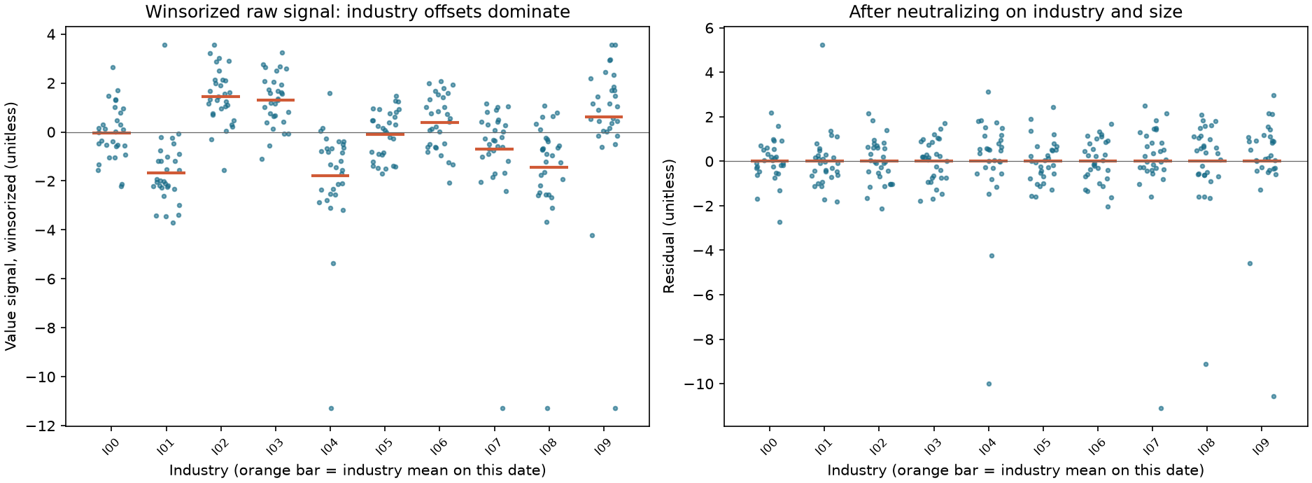
Winsorization removes most of the outlier variance; neutralization removes industry shifts and size loadings. This is the arithmetic behind “each step recovers some of the true IC.”

The assumptions matter: the disturbance must be unrelated to the label. If an industry shift itself predicts returns, it is not noise, and neutralization will remove it. Whether to neutralize is a research hypothesis and must be written into the plan.

6.3 Algebra of neutralization

All industry indicators. Let $D$ be the $n\times G$ industry-indicator matrix, with $G$ categories and exactly one category per stock. The solution to $\min_\alpha\|x-D\alpha\|^2$ is the within-group mean, so the residual is $e_i=x_i-\bar x_{g(i)}$: demean within group. Residuals sum to zero within each industry.

With a size control. Let $\tilde x$ and $\tilde c$ be signal and size after demeaning within industry. The Frisch–Waugh–Lovell theorem says that the residual from regressing $x$ simultaneously on $D$ and $c$ equals the residual from first removing the industry effect and then regressing $\tilde x$ on $\tilde c$:

The displayed division requires $\sum_i\tilde c_i^2>0$. If it is zero, size is already in the industry column space and adds no explanatory direction; the residual remains $\tilde x$, without division by zero. All steps must use the same valid-pair set.

Thus $e$ is orthogonal to size ($\sum_i e_i c_i=0$), and sums to zero within each industry.

Invariance under a redundant design. Adding a constant column (the sum of all industry indicators) makes the design matrix rank deficient. The residual is the projection of $x$ onto the orthogonal complement of the column space, so it depends only on the column space. Adding a redundant constant does not change that space; the residual is therefore independent of which column is dropped and of lstsq's minimum-norm choice. (In the test, residuals with and without a constant control column differ by less than $10^{-10}$.)

An industry with one stock. Its indicator uses a degree of freedom by itself, so its residual is always zero. If a date has too few valid names (fewer than 2 residual degrees of freedom), the row is NaN, not zero.

Relation to linear projection of weights. Let weights be $w=x$ (proportional to the signal), with constraint $Aw=0$, where the rows of $A$ are industry-indicator rows (possibly with an additional size-exposure row). Chapter 21's project_to_constraints computes $w-A^\top(AA^\top)^{-1}Aw$, which is exactly the OLS residual from regressing $x$ on the columns of $A^\top$. Thus, for weights proportional to the signal, “neutralize the signal, then take positions proportional to it” and “take positions proportional to the signal, then project” produce the same vector. Quantile weights (top quintile $+1/m$, bottom quintile $-1/m$) are a nonlinear function of the signal: taking quantiles after signal neutralization and projecting after taking quantiles produce different portfolios (see Section 10). Note that the sum of all industry-indicator rows is the dollar row, so do not add a separate dollar row (project_to_constraints requires linearly independent rows).

6.4 Composite IC and orthogonalization order

Assume $|r_{12}|<1$, so the residual variance is strictly positive, and that the label and signals are jointly feasible. For two standardized signals with label correlations $\rho_1,\rho_2$ and signal correlation $r_{12}$, the equal-weight composite $z_1+z_2$ has covariance $\rho_1+\rho_2$ and variance $2(1+r_{12})$. Its IC is $(\rho_1+\rho_2)/\sqrt{2(1+r_{12})}$; when $r_{12}=0$, this is Chapter 26's $(\rho_1+\rho_2)/\sqrt2$.

Sequential orthogonalization. Keep $z_1$ first, then regress $z_2$ on $z_1$ and take the residual $e_2=z_2-r_{12}z_1$ (variance $1-r_{12}^2$, uncorrelated with $z_1$). Standardize it to $\tilde e_2=e_2/\sqrt{1-r_{12}^2}$. Then $\mathrm{Cov}(\tilde e_2,y)=(\rho_2-r_{12}\rho_1)/\sqrt{1-r_{12}^2}$. Adding the two uncorrelated unit-variance signals gives

Reversing the order gives $\mathrm{IC}_{2\to1}=\frac1{\sqrt2}\bigl[\rho_2+(\rho_1-r_{12}\rho_2)/\sqrt{1-r_{12}^2}\bigr]$. The two generally differ. For $\rho_1=0.04,\rho_2=0.02,r_{12}=0.5$, the values are $\mathrm{IC}_{1\to2}=0.0283$, $\mathrm{IC}_{2\to1}=0.0386$, equal weight 0.0346, and optimal 0.0400 (below). In this example, $\rho_2=r_{12}\rho_1$: all of the second factor's predictive power comes from its correlation with the first. Once the first is removed, the second contains no incremental information; putting the first factor first and orthogonalizing the second leaves only the latter's noise.

$K$ signals. Require the correlation matrix to be positive definite, so each Cholesky residual variance is positive. Using the Cholesky factorization $PRP^\top=LL^\top$ (where $P$ permutes the order), the unit residuals from Gram–Schmidt are $L^{-1}Pz$, and their correlations with the label are $L^{-1}P\rho$. Thus the IC of their equal-weight combination after sequential orthogonalization is $\mathbf 1^\top L^{-1}P\rho/\sqrt K$ (sequential_orthogonal_ic).

IC-maximizing weights. Maximize $w^\top\rho/\sqrt{w^\top Rw}$. The Lagrange condition is $\rho=\lambda Rw$, so $w^*\propto R^{-1}\rho$ and the maximum IC is $\sqrt{\rho^\top R^{-1}\rho}$. In the example, $R^{-1}\rho=(0.04,0)$, which is proportional to $(0.04-0.5\times0.02,\ 0.02-0.5\times0.04)=(0.03,0)$. Thus, after normalizing, all weight goes to the first factor and the IC is $0.04=\rho_1$. This requires positive-definite $R$, nonzero $\rho$, and joint feasibility with the label. If $\rho=0$, every nonzero direction has IC zero, so there is no unique optimal direction and the zero vector cannot be normalized; the API raises an error. The true optimum formula uses true values; estimating them requires independent discovery-period data.

Interpretation. There is no “correct” order. Choosing the order with the highest evaluation-period IC is multiple testing (Chapter 22). A defensible approach is to state in advance that the economically most basic factor comes first and to record all order variants in the ledger.

6.5 Weight choice and tuning optimism

Equal weights require no estimation. Weights proportional to discovery-period IC, $\hat w_k\propto\max(\widehat{\mathrm{IC}}_k,0)$, require estimating each factor's mean IC. With $T$ months and $n$ names per month, the standard error of mean IC is about $1/\sqrt{nT}$ (for independent dates; each day's IC is approximately $1/\sqrt n$). At $n=300,T=60$, this is 0.0075. In the constructed panel, true ICs for value, momentum, and quality are 0.014, 0.049, and 0.033. Estimation noise is as large as value's true IC, so estimated weights can randomly push it to zero or inflate it. Choosing the best performer by the same discovery-period measure is optimistic in expectation across repeated samples due to selection bias; an individual realization need not be optimistic. The IC-proportional rule also does not exactly maximize discovery-period composite IC and is not guaranteed to beat equal weights in a holdout. Across 60 new worlds in Section 10, IC-proportional discovery weights beat equal weights in the holdout in only 31.7% of worlds; the “best discovery-period single factor” did so in 3.3%.

6.6 Missing factors: whose scale changed?

Suppose there are $K$ standardized, equally weighted signals. A name has $k$ available factors. Here $\bar r$ is the average pairwise correlation within that available subset, and we assume the subset signals still have unit variance in the conditional distribution under discussion. If missingness depends on signal value or label, the complete-population moments below cannot be carried over unchanged.

Reweight over available factors: $c=\frac1k\sum_{j\in\mathrm{available}}z_j$, with variance $\frac1{k^2}[k+k(k-1)\bar r]=\frac{1+(k-1)\bar r}{k}$. When $\bar r=0$, this is $1/k$; when $\bar r<0$, it lowers the average's variance further than the independent case. For example, with $k=2$ and $\bar r=-0.5$, the variance is 0.25, below 0.5 under independence. The correlation structure must be feasible and the resulting variance nonnegative. Zero fill: $c=\frac1K\sum_{j\in\mathrm{available}}z_j$, with variance $\frac{k}{K^2}[1+(k-1)\bar r]$.

For the constructed panel's three factors, $\bar r=(-0.3-0.3+0.2)/3=-0.133$. Names with all three factors have composite variance $(1+2\times(-0.133))/3=0.244$ (standard deviation 0.49). A name with only one factor has variance 1 under reweighting (standard deviation 1, or 2.0 times the complete-name standard deviation) and variance $1/9$ under zero fill (standard deviation 0.33, or 0.67 times the complete-name standard deviation). Without restandardizing, reweighting gives names with fewer factors greater variance, while zero fill compresses their scale. Variance alone cannot establish tail probabilities for arbitrary distributions. The tail shares below are observed in this construction under its specified missingness mechanism. In Section 10, these names are 5.7% of valid names; under reweighting they account for 8.8% of the top quintile, and under zero fill for 3.5%.

Missingness mechanism. Under missing completely at random (MCAR), the scale comparison above applies to the corresponding subset moments. If missingness depends on the signal (for example, loss-making companies lack a profitability ratio), conditional moments may also change; bias is not necessarily mild or larger. This chapter simulates only random missingness. Recommended practice: set a minimum number of factors (such as 2), report coverage, run sensitivity checks for both treatments, and record variants in the ledger.

6.7 Look-ahead in time-series standardization

Standardizing each stock's signal time series using the full-sample mean and standard deviation makes row $t$ depend on data after $t$. Counterexample: for a stock's signal sequence $(1,2,3,10)$, at the third observation $t=3$, the past-only expanding version (mean 2, standard deviation 1) gives $z=(3-2)/1=+1.0$; the full sample (mean 4, standard deviation 4.08) gives $z=(3-4)/4.08=-0.245$. The sign flips solely because the future value 10 enters the full-sample mean. Rule: every transform in row $t$ uses only rows $\le t$. Test by changing the last row; earlier outputs must not change (expanding_zscore has this test). Same-date cross-sectional transforms use only the current row, but point-in-time eligibility also requires that the input version and policy for that row were known at the time.

6.8 Factor correlation, diversification, and unstable correlations

For an equal-risk average of $k$ factors, each with Sharpe ratio $S=\mu/\sigma$ and average pairwise correlation $\bar\rho$, the portfolio mean is $\mu$ (the equal-weight average), and variance is $\sigma^2[1+(k-1)\bar\rho]/k$. Therefore,

When $\bar\rho=1$, $S_p=S$ (no diversification); when $\bar\rho=0$, it is $S\sqrt k$. The correlation matrix must be positive semidefinite, so $\bar\rho$ cannot be below $-1/(k-1)$. At that lower bound, portfolio variance is zero and the Sharpe ratio is undefined (diversified_sharpe requires a value strictly above the bound). Examples for $S=0.3,k=3$: $\bar\rho=0$ gives 0.520; 0.2 gives 0.439; 0.8 gives 0.322.

If the factors have equal risk but different Sharpe ratios, replace $S$ in the numerator with their average Sharpe ratio; this requires component standard deviations to be equal under the same evaluation convention. Scaling by past volatility does not guarantee equal realized risk in the future evaluation sample.

Correlation is estimated. Under an i.i.d. approximately bivariate-normal model and a large-sample approximation, the standard error of the sample correlation from $T$ monthly observations is about $(1-\rho^2)/\sqrt T$ when the true correlation is $\rho$. At $T=60,\rho=0$, this is 0.13. A correlation matrix estimated from 60 months can therefore move substantially; in Section 11, HML and RMW (published value and quality factors) have opposite signs in 1963–1999 and 2000–2026.

6.9 Crowding: definition and what can be measured

Measuring crowding requires knowing how much capital holds similar positions, which calls for holdings, short-borrow rates, fund flows, and similar data. This chapter has none of those, so it can do only two things: (i) measure signal-level position overlap as the intersection share of two factors' same-date top-quintile names; under independence this should be 0.20; and (ii) measure return-level synchronicity using factor-return correlations and rolling correlations. The first is calculated in the constructed panel (value/momentum 0.10, value/quality 0.10, momentum/quality 0.28); the second uses published factor returns (Section 11). Neither establishes “crowding”; each is only one observable aspect of it.

6.10 Projection on the support set: who is neutral, and when?

The support set $\mathcal S_t=\{i:\mathrm{listed}_{i,t}=\mathrm{True}\}$ contains names listed at signal month-end. The alpha-valid set is the subset with nonmissing composite scores; the two are not the same. First form fixed top-quintile long-short weights $w^0$ on the alpha-valid set; weights outside the support set must be zero. An optional industry projection may use names in $\mathcal S_t$ that have no valid score to carry hedge weights. The resulting portfolio is no longer a pure top/bottom-score-quintile portfolio, and that must be disclosed.

Let $u=w^0_{\mathcal S_t}$, and let $A_t$ contain industry-indicator rows only for names in that support set, with every name assigned to exactly one nonmissing industry. Construct only independent rows; their sum is already the net-position row, so do not add it again. If each row has at least one coordinate, $A_tA_t^\top$ is a positive diagonal matrix of industry counts. The support-set form of Chapter 21's nearest-point projection is

Projecting the full-column weights first and then zeroing unlisted names generally differs from this formula: masking deletes coordinates that used to offset industry net positions. If an industry has only one listed name, its constraint sets that name's weight to zero; this is not rank deficiency of the full matrix, but the absence of any nonzero hedge direction in that industry. An empty support set, no initial long-short portfolio, or a numerically zero projection must explicitly result in cash. Missing classifications or misaligned axes must fail explicitly; do not silently replace invalid inputs with zero.

Gross exposure and homogeneous constraints. If $g_v=\sum_{i\in\mathcal S_t}|v_i|$ is above the numerical-zero threshold, set $k=2/g_v>0$, $w_{\mathcal S_t}=kv$, and all other coordinates to zero. Then $A_t(kv)=kA_tv=0$; industry net positions and total net position remain zero, gross exposure returns to 2, long exposure is 1, and short exposure is $-1$. If $g_v$ is only rounding noise, do not amplify it to 2. Projection gives the nearest point; the final result after rescaling is generally no longer the original nearest point. Restoring gross changes the position budget, not the return parameters. For a nonzero target $A_tv=b$, $A_t(kv)=kb$; unless $k=1$ or $b=0$, this proof does not apply. Current P4 adds no nonzero-target strategy.

Two thresholds. P4's min_names_per_date=60 counts $|\mathcal S_t|$, not the number of nonmissing values in each field. With 59 names, the date is ineligible for preprocessing and the portfolio holds cash. Sixty names opens universe eligibility only: a field still needs 30 values for winsorization, at least 10 residual values for a z-score, at least one field within a style, and at least two styles across the composite. No later combination may restore a date that failed eligibility; the portfolio entry point checks the 60-name requirement again so externally supplied scores cannot bypass it.

Clock and residuals. At month-end $t$, use then-listed status and signals to form a target. At $t+1$, delisting cancellations or liquidations, partial fills, and price drift can all cause actual holdings to differ from the target. Report separately: target weights outside the signal-time support set, industry net positions, total net, and gross; the same quantities after execution-target filtering; and actual closing holdings normalized by current NAV. Post-execution information may be used for execution and diagnosis, but cannot be written back into the month-$t$ scores or support set. Current P4 listing status is a constructed input; it has no real halt status, name-level price-availability, or borrow fields. A name marked listed is not necessarily truly tradable.

7. Financial interpretation

Preprocessing removes components unrelated to returns; it is not signal beautification. At each step, ask whether the removed component is really noise. Industry shifts, size loadings, and outliers are noise in the constructed panel, so each step recovers some IC (single-world momentum Pearson IC: 0.027 raw, 0.038 after winsorization, 0.048 after neutralization, versus true value 0.053). If a “disturbance” actually carries return information (real industry momentum or a size effect), preprocessing removes it.

Combination gains come from diversification, not magic. The benefit of adding two correlated factors is limited by their correlation; the composite-IC formula shows why. If all of one factor's predictive power comes from its correlation with another, it adds no incremental information.

Order and weights are researcher degrees of freedom. Orthogonalization order, weight choice, missing-factor treatment, and winsorization quantiles can all look “better” or “worse” in the evaluation period. Fix these choices in advance, record all variants, and evaluate tuning on an independent holdout.

Neutralization and constraints. For linear weights, signal neutralization and weight projection agree; for quantile weights, they differ. Therefore, “industry neutral” must say which operation was used: neutralize the signal and then rank, or rank and then project the weights. The two have different exposures, volatility, and turnover (Section 10).

Correlation is unstable. The correlation between published value and quality factors has opposite signs in different 20–30-year periods. Choosing weights from an estimated correlation matrix therefore relies on an estimate that can change sign. The diversification arithmetic (the $S_p$ formula) is conditional on average correlation, which itself changes.

8. Numerical examples: work through each step

All values are produced by hand_examples() and independently checked by qa/a5/claude/recompute/ch28_recompute.py. The stocks and signals are teaching constructions.

8.1 Winsorization, z-scores, and normal scores

On one date, 11 stocks have signals $1,2,\dots,10,100$ (the last is an outlier).

• Z-scores without winsorization: mean $155/11=14.09$, standard deviation $28.64$. The outlier's $z=(100-14.09)/28.64=3.00$; the other ten are compressed between $-0.457$ (signal 1) and $-0.143$ (signal 10), making them hard to distinguish.
• Winsorization (10th and 90th percentiles, linear interpolation): $(n-1)q=10\times0.1=1$ and 9, which are the 2nd and 10th order statistics, so $q^-=2$ and $q^+=10$. Values become $2,2,3,4,5,6,7,8,9,10,10$, with mean $66/11=6$. The sum of squared deviations is $16+16+9+4+1+0+1+4+9+16+16=92$; sample variance is $92/10=9.2$ and standard deviation is $3.033$. Signals 10 and 100 both have $z=+1.319$; signal 5 has $z=-0.330$, slightly below its un-winsorized value of $-0.317$, but the ten ordinary names now span $-1.32$ to $+1.32$.
• Normal scores: $\Phi^{-1}((r-1/2)/11)$. Signal 100 (rank 11) gets $\Phi^{-1}(10.5/11)=1.691$; signal 10 (rank 10) gets $\Phi^{-1}(9.5/11)=1.097$. Magnitudes are discarded; only ranks remain.

8.2 Industry neutralization: reversing the sign

There are six stocks: industry A is $\{a,b,c\}$ and industry B is $\{d,e,f\}$. Signal $x=(1,-1,0,\ 11,10,9)$ and next-month returns $y=(5\%,3\%,4\%,\ -3\%,-4\%,-5\%)$. Industry B has a higher overall signal (shift of 10) and lower returns, while within each industry a higher signal corresponds to a higher return.

• Raw Pearson IC: $\bar x=30/6=5$, $x-\bar x=(-4,-6,-5,6,5,4)$, $\sum(x-\bar x)y=-1.16$, $\sum(x-\bar x)^2=154$, and $\sum y^2=0.01$. Thus IC $=-1.16/\sqrt{154\times0.01}=-0.935$.
• After neutralization: industry means are 0 and 10, so residuals are $e=(1,-1,0,\ 1,0,-1)$ and sum to zero within each industry. $\sum ey=0.04$, $\sum e^2=4$, so IC $=0.04/\sqrt{4\times0.01}=+0.200$.

The industry shift is unrelated to the within-industry ordering but points opposite to the industry return. Before neutralization, IC is $-0.94$; afterward it is $+0.20$.

8.3 Linear-constraint projection and neutralization produce the same vector

Use $x$ from 8.2 again, with weights $w=x$. Let the two rows of constraint matrix $A$ be the indicators for industries A and B (their sum is the dollar row, so do not add it again). $AA^\top=\mathrm{diag}(3,3)$, $Ax=(0,30)$, and $w-A^\top(AA^\top)^{-1}Ax=x-(0,0,0,10,10,10)=(1,-1,0,1,0,-1)$. This matches the 8.2 residual exactly. After projection, total net position and each industry's net position are zero. This holds for weights proportional to the signal, not quantile weights. In Section 10, the mean maximum industry net position is 0.053 after neutralizing the signal and taking quintiles, but zero after taking quintiles on the raw composite and projecting the weights.

8.4 Two correlated signals: equal weights, two orthogonalization orders, and the optimum

8.5 Missing factors

Two factors have weights $(0.5,0.5)$. Name $s_1$ has both factors, $z=(2,2)$, and composite 2.0. Name $s_2$ has only the second factor, $z=1$:

• Reweight over available factors: $0.5\times1/0.5=1.0$ (preserves the z-score scale).
• Zero fill: $0.5\times1/1.0=0.5$ (shrunk toward 0).

Section 6.6 gives the broader example: for three factors with average correlation $-0.133$, complete names have composite standard deviation 0.49; names with one factor have standard deviation 1 after reweighting (2.0 times larger) and 0.33 after zero fill (0.67 times as large).

8.6 Look-ahead in standardization

A stock's signal sequence is $(1,2,3,10)$. At the third observation, using only the past $\{1,2,3\}$ (mean 2, standard deviation 1) gives $z=+1.0$; the full sample (mean 4, standard deviation $4.082$) gives $z=(3-4)/4.082=-0.245$. The sign reverses because the full-sample mean uses the future value 10.

8.7 Diversification

Three factors each have Sharpe ratio 0.3. Average correlation 0 gives $0.3\sqrt3=0.520$; 0.2 gives $0.520/\sqrt{1.4}=0.439$; 0.8 gives $0.520/\sqrt{2.6}=0.322$. The correlation matrix $\begin{pmatrix}1&0.2&0.4\\0.2&1&0\\0.4&0&1\end{pmatrix}$ has average pairwise correlation $(0.2+0.4+0)/3=0.2$.

8.8 Three-coordinate support set in a four-name universe: counterexample to project-then-mask

There are four names a, b, c, d; industry A is a, b, and industry B is c, d. The weights $w=(0.4,-0.4,0.3,-0.3)$ are neutral over the full set and have gross exposure 1.4. Suppose a is not listed at signal time. Projecting as before (the weights do not change), then zeroing a, gives $(0,-0.4,0.3,-0.3)$: industry A net $-0.4$, total net $-0.4$, and gross 1.0. An unlisted name is not a negligible implementation detail.

The correct support set is $(b,c,d)$, with original vector $u=(-0.4,0.3,-0.3)$:

Subtracting the industry means gives $v=(0,0.3,-0.3)$, gross 0.6. Multiplying by $2/0.6=10/3$ gives final weights $(0,0,1,-1)$ (embedded back into the full column set). The unlisted a has weight zero; the sole name in industry A, b, is also forced to zero; industry B net and total net are zero; gross is 2. The budget is restored, but the original four quantile positions are not preserved.

Now consider a missing-alpha hedge coordinate. All four names are listed, but only a and c have scores, with initial long-short weights $(1,0,-1,0)$. The two industry means are $0.5$ and $-0.5$, so projection gives $v=(0.5,-0.5,-0.5,0.5)$, already with gross 2. Names b and d have no score but carry hedge positions. This is the declared optional projection semantics; it does not invent alpha values for missing names. If only a and c are listed and each is the sole name in its industry, projection is zero and the portfolio holds cash; do not divide by zero or scale noise to “restore gross.”

For contrast, use a nonzero target: industry A has one coordinate and requires $v_a=0.2$. Even if the projection satisfies the constraint, multiplying by 2 changes the target to 0.4. A nonzero target requires resolving the constrained problem; it cannot be scaled without qualification. All calculations in this section are independent hand examples, not new market results.

9. Python implementation

Functions are in the new module factor_preprocessing.py; ranking, IC, and quantile weights reuse Chapter 23's factor_research.py; linear-constraint projection reuses Chapter 21's project_to_constraints.

The default offline reading entry point is the accepted reader package's notebooks/ch28_multifactor.ipynb: RUN_FRENCH=False; it constructs 300 names by 120 months (seed 20261121), and the default tuning sweep uses 60 worlds. Create a new RUN_DIR only; do not write historical plots/CSV/JSON. The French analysis and four figures in this chapter are existing historical evidence and are not rerun by the default path. The runner also saves an execution copy and state. Code blocks are retained in full for study; the following are historical CLI/test entry points from the original project, not reader defaults. Do not run them when the isolated package does not include these project entry points:

.venv/bin/python code/ch28_multifactor.py
.venv/bin/python -m pytest tests/test_ch28_preprocessing.py tests/test_ch28_workflow.py -q

Frequency: monthly; signal_time is month-end; each row $t$ of same-date transforms uses only row $t$; expanding_zscore for row $t$ uses only rows $\le t$. Seeds: constructed panel 20261121; 60 new worlds starting at 20261122.

Code block one: winsorization, z-scores, and normal scores (Section 8.1).

import numpy as np
import pandas as pd

from quant_course.factor_preprocessing import normal_scores, winsorize_cross_section, zscore_cross_section

x = pd.DataFrame([[1.0, 2, 3, 4, 5, 6, 7, 8, 9, 10, 100]], index=pd.period_range("2026-06", periods=1, freq="M"))
w = winsorize_cross_section(x, lower=0.1, upper=0.9, min_names=10)
assert w.iloc[0].tolist() == [2, 2, 3, 4, 5, 6, 7, 8, 9, 10, 10]
assert abs(w.iloc[0].mean() - 6.0) < 1e-12 and abs(w.iloc[0].std(ddof=1) - np.sqrt(9.2)) < 1e-12
z_raw, z_win = zscore_cross_section(x), zscore_cross_section(w)
assert abs(z_raw.iloc[0, 10] - 3.0) < 0.001 and z_raw.iloc[0, :10].between(-0.46, -0.14).all()   # the ten ordinary names are squeezed together
assert abs(z_win.iloc[0, 9] - 4 / np.sqrt(9.2)) < 1e-12 and abs(z_win.iloc[0, 9] - z_win.iloc[0, 10]) < 1e-12
ns = normal_scores(x)
assert abs(ns.iloc[0, 10] - 1.6906) < 1e-4 and abs(ns.iloc[0, 9] - 1.0968) < 1e-4

Code block two: industry neutralization and linear-constraint projection (Sections 8.2 and 8.3).

import numpy as np
import pandas as pd

from quant_course.factor_preprocessing import neutralize
from quant_course.portfolio_construction import project_to_constraints

cols = list("abcdef")
sig = pd.DataFrame([[1.0, -1.0, 0.0, 11.0, 10.0, 9.0]], index=pd.period_range("2026-06", periods=1, freq="M"), columns=cols)
ret = np.array([0.05, 0.03, 0.04, -0.03, -0.04, -0.05])
groups = pd.Series(list("AAABBB"), index=cols)
res = neutralize(sig, groups=groups)
assert np.allclose(res.iloc[0], [1, -1, 0, 1, 0, -1], atol=1e-12)
assert abs(np.corrcoef(sig.iloc[0], ret)[0, 1] + 0.93475) < 1e-5 and abs(np.corrcoef(res.iloc[0], ret)[0, 1] - 0.2) < 1e-12
A = np.array([[1, 1, 1, 0, 0, 0], [0, 0, 0, 1, 1, 1]], dtype=float)         # industry indicator rows; their sum is the dollar row
proj = project_to_constraints(sig.iloc[0].to_numpy(), A)
assert np.allclose(proj, res.iloc[0], atol=1e-12) and abs(proj.sum()) < 1e-12 and np.allclose(A @ proj, 0)

Code block three: combining two correlated signals and order dependence (Section 8.4).

import numpy as np

from quant_course.factor_preprocessing import composite_ic, optimal_composite_weights, sequential_orthogonal_ic

R = np.array([[1.0, 0.5], [0.5, 1.0]])
rho = [0.04, 0.02]
assert abs(composite_ic(rho, R) - 0.06 / np.sqrt(3)) < 1e-12
a, b = sequential_orthogonal_ic(rho, R, [0, 1]), sequential_orthogonal_ic(rho, R, [1, 0])
assert abs(a - 0.04 / np.sqrt(2)) < 1e-12 and abs(b - (0.02 + 0.03 / np.sqrt(0.75)) / np.sqrt(2)) < 1e-12 and b > a
w, best = optimal_composite_weights(rho, R)
assert np.allclose(w, [1.0, 0.0]) and abs(best - 0.04) < 1e-12 and abs(composite_ic(rho, R, w) - 0.04) < 1e-12
assert best > b > composite_ic(rho, R) > a                                      # 0.0400 > 0.0386 > 0.0346 > 0.0283

Code block four: missing-factor scale (Sections 8.5 and 6.6).

import numpy as np
import pandas as pd

from quant_course.factor_preprocessing import combine_signals

idx = pd.period_range("2026-06", periods=1, freq="M")
z = {"f1": pd.DataFrame([[2.0, np.nan]], index=idx, columns=["s1", "s2"]), "f2": pd.DataFrame([[2.0, 1.0]], index=idx, columns=["s1", "s2"])}
rw, count = combine_signals(z, {"f1": 0.5, "f2": 0.5}, missing="reweight")
zero, _ = combine_signals(z, {"f1": 0.5, "f2": 0.5}, missing="zero")
assert rw.iloc[0].tolist() == [2.0, 1.0] and zero.iloc[0].tolist() == [2.0, 0.5] and count.iloc[0].tolist() == [2, 1]

rng = np.random.default_rng(0)
R = np.array([[1.0, -0.3, -0.3], [-0.3, 1.0, 0.2], [-0.3, 0.2, 1.0]])
full = rng.multivariate_normal(np.zeros(3), R, size=300_000)                      # three standardized factors, mean correlation -0.133
var3 = full.mean(axis=1).var()
assert abs(var3 - (1 + 2 * (-0.1333)) / 3) < 0.005                                # (1 + (k-1) r) / k with k = 3
reweighted_one, zero_filled_one = full[:, 0], full[:, 0] / 3                      # a name that has only the first factor
assert abs(reweighted_one.var() / var3 - 1 / 0.2444) < 0.15 and abs(zero_filled_one.var() / var3 - (1 / 9) / 0.2444) < 0.02

Code block five: look-ahead in standardization (Section 8.6).

import pandas as pd

from quant_course.factor_preprocessing import expanding_zscore

x = pd.DataFrame({"x": [1.0, 2.0, 3.0, 10.0]}, index=pd.period_range("2026-01", periods=4, freq="M"))
past = expanding_zscore(x, min_periods=3)
full = (x["x"] - x["x"].mean()) / x["x"].std(ddof=1)
assert abs(past["x"].iloc[2] - 1.0) < 1e-12 and abs(full.iloc[2] + 0.244949) < 1e-6   # opposite signs at the third observation
changed = x.copy(); changed.iloc[3, 0] = -100.0                                        # change only the last row
assert expanding_zscore(changed, min_periods=3)["x"].iloc[:3].equals(past["x"].iloc[:3])

Code block six: diversification (Section 8.7).

import numpy as np

from quant_course.factor_preprocessing import average_pairwise_correlation, diversified_sharpe

assert abs(diversified_sharpe(0.3, 3, 0.0) - 0.3 * np.sqrt(3)) < 1e-12
assert abs(diversified_sharpe(0.3, 3, 0.2) - 0.43916) < 1e-5 and abs(diversified_sharpe(0.3, 3, 0.8) - 0.32225) < 1e-5
assert abs(average_pairwise_correlation(np.array([[1, 0.2, 0.4], [0.2, 1, 0.0], [0.4, 0.0, 1]])) - 0.2) < 1e-12
assert abs(diversified_sharpe(0.3, 3, 1.0) - 0.3) < 1e-12                          # perfectly correlated: no diversification

10. Reading the figures

Constructed panel. 300 stocks, 120 months (119 months with labels), seed 20261121. Three true signals (value, momentum, quality), with same-date correlations $-0.3,-0.3,0.2$. Next-month returns load on the true signals by $(0.0030,0.0040,0.0025)$, plus a common industry shock (standard deviation 2%) and idiosyncratic noise (7%). Observed raw signals equal true signals plus industry shifts (for every factor and industry, an AR(1) process with coefficient 0.9 and variance 1), size loadings ($-0.5,0,0.3$), and outliers with probability 2% and standard deviation 8. The analytic correlations between true signals and labels are 0.0144 for value, 0.0493 for momentum, and 0.0329 for quality (return standard deviation 7.30%). This is a known data-generating process, not market evidence.

Figure 28-1: Winsorization and stepwise recovery of IC. Left: histogram (log vertical axis) of one day's value signal; orange is raw (with outliers at $-12$ and $+6$), blue is winsorized at the same-date 1st/99th percentiles. Right: mean monthly IC over five treatments for each factor (119 months): raw Pearson, winsorized Pearson, winsorized plus neutralized Pearson, winsorized plus neutralized Spearman, and true-signal Pearson. Momentum rises from 0.027 to 0.038 to 0.048, versus true value 0.053. Quality is 0.025, 0.028, and 0.031, versus true value 0.032. Value's IC is small (true value 0.014; sampling error in one world is about 0.005), so its trend is not visible in one world; see the average over 60 new seeds below.

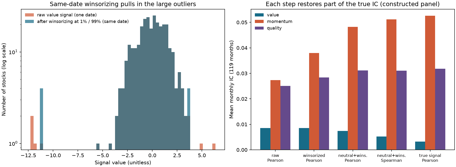
Mean Pearson IC and attenuation across 60 new worlds (raw, after winsorization, and after neutralization plus winsorization, relative to the true signal).

Figure 28-2: Cross-section before and after neutralization. Left: one day's winsorized value signal plotted by industry. Right: residuals after neutralizing industry and size. Orange horizontal lines show the same-day industry means. On the left, industry means are visibly separated (industry shifts explain much of the signal variation); on the right, each industry's mean is zero (the largest absolute industry mean on one date is $1.9\times10^{-15}$, and residual/size correlation is $-1.0\times10^{-17}$). Several points remain at $-9$ to $-11$: these are outlier stocks that were winsorized at $-11.3$ before neutralization, so they remain outliers afterward. Removing them would require a second winsorization after neutralization, which is another variant to record in the ledger.

Combination (Pearson IC, 119 months; values in parentheses are analytic values using the true signals and true correlation matrix).

The best analytic single-factor IC is 0.0493. Order changes IC from 0.0595 to 0.0661 analytically, with measured IC moving in the same direction. Measured Pearson IC is 0.008–0.010 below the analytic value. About 0.006 is sampling variation in this world: an equal-weight combination of the true signals has measured Pearson IC 0.0590 ($t=11.7$), 0.006 below the analytic 0.0651, with a standard error of about 0.005. Another 0.003 is additional loss from using processed signals rather than the true signals (winsorization and neutralization also remove some true signal).

Figure 28-3: Combination and tuning. Left: mean Pearson IC for combinations of the same three processed signals (horizontal bars show $\pm2$ standard errors); red dashed line marks the analytic optimum, 0.0665. Right: in 60 new worlds, weights estimated from the first 60 discovery months (orange) and the best discovery-period single factor (purple) are evaluated over the next 59 holdout months as IC minus equal-weight holdout IC. Orange values cluster on both sides of zero, more often negative (positive in only 31.7% of worlds); purple values are almost all negative (positive in 3.3%).

The red line is the oracle optimum under the stipulated population DGP moments, not a hard upper bound on every finite-sample measured IC. Likewise, Figure28-1’s “stepwise recovery” describes the specified disturbance mechanism and reported averages; it does not guarantee a monotone increase for value at every step in a single world.

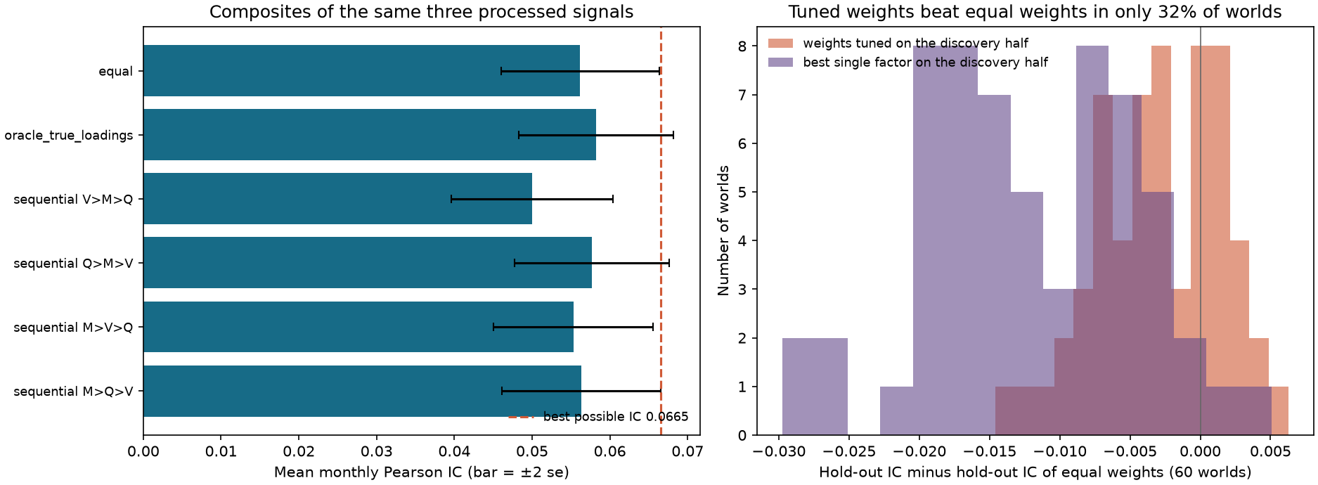
Mean discovery- and holdout-period Spearman IC across 60 new worlds.

Missing factors (15% random missingness for each processed factor; one world, 119 months).

Interpretation: IC differences are small under random missingness, and the dropped-name treatment uses a different name set, so the numbers are not directly comparable. Scale bias is visible in top-quintile membership: reweighting makes single-factor names appear 1.55 times as often (8.8% versus 5.7%); zero fill reduces their representation to 0.62 times as often.

Constraints (one world, 119 months, gross returns before costs).

The projected portfolio has exactly zero industry net and the lowest volatility (0.93%), so it has the highest $t$-statistic. Its average return is below that of the neutralized-signal quintile portfolio. These are different portfolios: projection means the weights are no longer “$+1/m$ in the top quintile and $-1/m$ in the bottom quintile.” The comparison is in one constructed world and does not establish which method is better; it shows that they differ and must be identified. Position overlap: top-quintile intersection is 10.3% for value/momentum, 10.4% for value/quality, and 27.7% for momentum/quality (20% under independence).

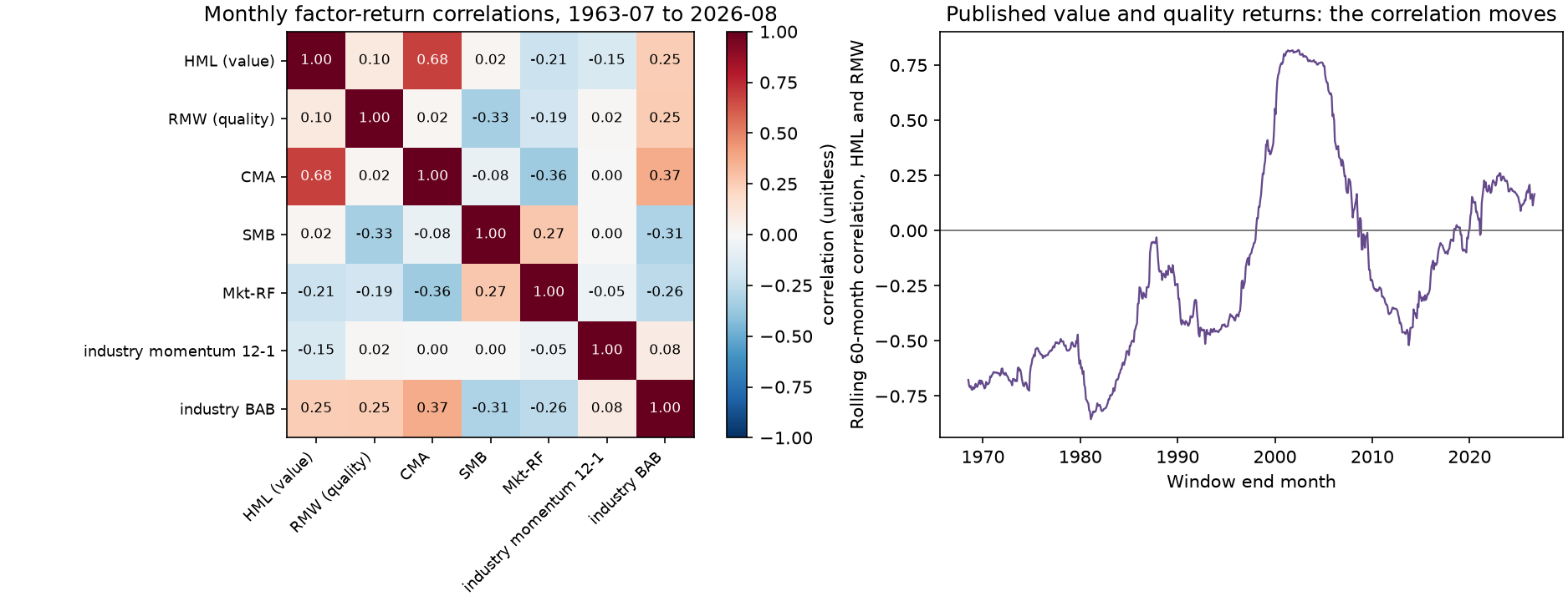
Figure 28-4: Correlations among published factor returns. Left: monthly return correlation matrix for the five FF5 factors and two strategies constructed from 10 industry portfolios (cross-sectional momentum 12–1 and BAB), from 1963-07 through 2026-08 (758 months). Right: rolling 60-month correlation between HML and RMW. The rolling correlation ranges from $-0.85$ (1981-01) to $+0.82$ (2002-05). On the left, HML/CMA correlation is 0.68, HML/RMW is 0.10, and industry momentum/HML is $-0.15$.

11. Real-market example

Data and limits. This uses the French five-factor (2×3) monthly data frozen on 2026-10-05 (processed CSV SHA-256: 833bd925b49651428781c789c13a6ac7454d4676449e6d119782050046a57eea; 758 months, 1963-07 through 2026-08), plus the French 10-industry and FF3 snapshots used in Chapters 25 and 27 (see Chapter 25 source notes for processed hashes). Factor construction follows the French database's five-factor description: HML is one-half (Small Value + Big Value) minus one-half (Small Growth + Big Growth); RMW and CMA (conservative minus aggressive investment) are formed similarly. These are published aggregate returns, not stock-level signals, point-in-time versions, or executable trades. The two “industry strategies” are built from 10 value-weighted industry portfolios: cross-sectional 12–1 momentum (quintiles, two industries per bucket, $K=1$) and BAB (60-month beta, shrinkage 0.6). They are neither the published UMD and BAB factors nor individual-stock strategies. Return months are aligned on the common period 1963-07 through 2026-08.

Correlation matrix (758 months).

Unstable correlation. HML/RMW correlation is 0.095 over the full sample; $-0.335$ from 1963-07 through 1999-12; and $+0.337$ from 2000-01 through 2026-08. Rolling 60-month correlation ranges from $-0.855$ (window ending 1981-01) to $+0.818$ (ending 2002-05); the latest window is 0.165. The two subperiods use the date split carried over from Chapters 23–27; they were not selected for this chapter.

Equal-risk average. Take the monthly return series for HML, RMW, and industry momentum; divide each by its own expanding standard deviation through the prior month (at least 60 months, using only data through $t-1$; drop the first 60 months), then average. Over 698 months (1968-07 through 2026-08), annualized component Sharpe ratios are 0.341 (HML), 0.380 (RMW), and 0.294 (industry momentum), for an average of 0.338. Average pairwise correlation is $-0.035$. The equal-risk average has a Sharpe ratio of 0.608. Substituting the average component Sharpe into the simplified equal-risk formula, $S\sqrt3/\sqrt{1+2\bar\rho}$, also rounds to 0.608. The unrounded portfolio estimate is 0.6077680037077575; the simplified formula gives 0.6079788525663137, a difference of about 0.00021085. Expanding scaling by past risk does not force realized standard deviations to be exactly equal over these 698 months, so the close match is an approximation, not an identity. Full-sample standard deviation scaling (which looks ahead) gives a Sharpe ratio of 0.590 over the same months. Interpretation: the diversification arithmetic is close in-sample; look-ahead scaling did not raise the Sharpe in this sample, but it was unavailable at signal_time and is not a usable method. The numerical closeness is specific to this dataset.

What can and cannot be said. We can say that the published value and quality factors have opposite correlations across subperiods from 1963 through 2026, illustrating short-window estimation uncertainty and cross-period drift; this does not imply that every 60-month matrix is necessarily unstable. We can also say that the in-sample Sharpe of an equal-risk average of three low-correlation return series is close to the simplified formula. We cannot say: (1) that this portfolio has a 0.6 Sharpe out of sample; the value uses three components and 698 in-sample months, HML and RMW are published revised histories, and industry momentum uses only 10 industries; (2) that value and quality factors are “crowded,” because this chapter has no holdings, short-borrow rates, or fund-flow data; (3) how a stock-level multi-factor portfolio performs, because the stock-level experiment here is only a constructed panel; or (4) anything about costs, capacity, or tradability.

12. Common errors

Error 1: Standardizing with a full-sample fit. Using full-sample mean and standard deviation for each stock's time series makes row $t$ depend on the future (Section 8.6: $+1.0$ versus $-0.245$). Fix: use same-date cross-sectional z-scores or an expanding version; test that changing the last row leaves earlier outputs unchanged (code block five).

Error 2: Winsorizing with quantiles from the entire panel. Pooling all dates to calculate the 1st and 99th percentiles uses other dates' distributions, including the future. Fix: compute cross-sectional quantiles separately for each date (winsorize_cross_section).

Error 3: Choosing winsorization or z-score parameters by evaluation-period IC. The choice of quantiles (1%/99% or 5%/95%), degrees of freedom, and a second winsorization can all look different in the evaluation period. Fix: specify them in advance and record variants in the ledger (Chapter 22).

Error 4: Neutralizing with hindsight industry labels. Industry classifications can be revised; a label unavailable at signal_time introduces future information. Fix: use the version known at the time (date-indexed groups) and report the share of missing labels.

Error 5: Removing true signal through neutralization. If an industry shift itself carries returns (real industry momentum or a value effect), neutralization removes it. Fix: state whether neutralization is a research hypothesis and report IC before and after; do not transfer a favorable constructed-world result to real data.

Error 6: Using too many controls. Every added control consumes degrees of freedom; on a date with eight stocks, ten industry indicators leave no residual variation. Fix: return NaN when degrees of freedom are insufficient (the neutralize rule) and report how many dates were dropped.

Error 7: Confusing signal neutralization with linear-constraint projection. They agree for weights proportional to the signal (Section 8.3) and differ for quantile weights (Section 10: mean maximum industry net is 0.053 versus $5\times10^{-17}$, with different volatility and returns). Fix: identify which operation was used.

Error 8: Choosing orthogonalization order after evaluation. Order can change IC by 36% (Section 8.4). Fix: state a rule in advance, such as “the foundational factor comes first,” and record all orders.

Error 9: Choosing composite weights from evaluation-period performance. Discovery-period IC-proportional weights beat equal weights in the holdout in only 31.7% of worlds (Section 10); the best single factor does so in 3.3%. Fix: fix weights in advance, or estimate them in discovery and evaluate them in an independent holdout, with the process recorded.

Error 10: Failing to report coverage and scale after zero fill or reweighting. In this constructed random-missingness sample, reweighting makes single-factor names appear in the top quintile 1.55 times as often as their baseline share; zero fill pushes them toward the middle (0.62 times). Fix: set a minimum factor count, report coverage and the single-factor share, and test sensitivity to both treatments.

Error 11: Configuring weights from one 60-month correlation matrix. HML/RMW correlation is $-0.34$ in 1963–1999 and $+0.34$ in 2000–2026, with a rolling range from $-0.86$ to $+0.82$ (Section 11). Fix: report estimation uncertainty and multiple periods; state that the diversification formula depends on average correlation.

Error 12: Confusing signal correlation with return correlation. Signal correlation (same-date cross-section) determines composite IC; return correlation (time series of factor returns) determines diversification. Their signs can differ (constructed panel: signal correlations of $-0.3$, while all true signals have positive next-month return loadings).

Error 13: Treating position overlap as proof of crowding. Top-quintile overlap is only one aspect; assessing crowding requires holdings, short-borrow, and fund-flow data (Section 6.9).

13. Quant research application

Multi-factor workflow contract (Project 4 signal layer).

Research workflow (constructed panel with known data-generating process). Frozen plan: hypothesize that “the equal-weight composite of three processed factors has positive same-date Rank IC with next-month returns and exceeds each single factor's IC”; primary measure is the composite's mean Rank IC and its $t$-statistic. Preprocessing is fixed as 1%/99% winsorization, neutralization by industry and size, and z-scoring; weights are fixed at equal weight. Result: composite Rank IC is 0.0519 ($t=10.5$), slightly above momentum's 0.0511, but the composite's own $t$-statistic does not test the difference between the two. Supporting “better than any single factor” requires a separate paired, same-month difference evaluation; that additional test is not in this batch. Pearson IC is 0.0562. Sequential-orthogonalization IC ranges from 0.0467 to 0.0532, depending on order; missing-factor IC ranges from 0.0458 to 0.0511. Across 60 new worlds, discovery-period tuning beats equal weights in the holdout in only 31.7% of worlds. The construction provides checkable expectations. These results provide limited engineering evidence about the tested inputs and workflow; they do not prove correctness for arbitrary inputs and are not real-world effects.

Variants in the ledger. Winsorization (yes/no) × neutralization (yes/no) × combination (equal weight, true loadings, four sequential orders) × missing-data treatment (four options) × constraint (three options). Not every combination was evaluated, but every evaluated variant must be recorded; all reported $t$-statistics are naive and unadjusted for multiple testing.

Constraints for Project 4. (1) Use only data available by the signal month; same-date transforms use that date's cross-section. (2) Use industry labels known at the time. (3) Fix weights, winsorization quantiles, minimum factor count, and orthogonalization order in advance. (4) Report coverage per factor and composite, shares of dropped or imputed names, and the share of single-factor names at both tails. (5) Report IC before and after neutralization, plus industry and size exposures. (6) State whether the constraint is signal neutralization or weight projection. (7) Report correlation uncertainty and values for multiple periods. (8) Do not claim “crowding” without actual holdings data.

13.1 How to read the C13 protocol correction alongside historical results

The original constructed panel, figures, and French aggregate diagnostics in Sections 9–11 remain tied to their own inputs; they are not rewritten as a new P4 run. The old A5/A6 P4 projected over all 240 columns and then filtered by listing status. Its historical record includes 1,842 name-months zeroed out and a maximum industry net position of 0.0280748663 after filtering. This exposed a mismatch between protocol and implementation; a claim that “industry projection was already applied” does not replace a support-set check.

C13 corrected the protocol while preserving the meaning of the original configuration: enforce the 60-name threshold at preprocessing and portfolio entry; apply optional industry projection only on the signal-time listed support set; restore configured gross of 2 after the homogeneous projection; explicitly record degenerate cases as cash; and report A6 target and actual-holding residuals separately. The original seven fields, ranking and combination formulas, data-generating process, seed, and two frozen configurations are unchanged. The new source hashes, old/new sample, weight, return, and cost differences, and checks are documented in the accepted P4 protocol-alignment note.

This correction is a normative alignment made after the old results had been seen. It is not a new blind preregistration, independent market test, or tuned strategy. Keep favorable and unfavorable return changes. Restoring configured gross and neutrality does not establish alpha, borrow availability, or capacity. Chapter 29 remains responsible for execution ledgers and cash/fee reconciliation; execution-day states do not flow backward into the signal.

14. Chapter summary

A multi-factor workflow has three layers: preprocessing (same-date cross-sectional transforms that change scale, outliers, and unwanted exposures), combination (weights fixed in advance), and constraints (portfolio-level exposures). When a signal contains a component unrelated to returns, Pearson IC is attenuated by $1/\sqrt{1+\sigma_u^2/\sigma_s^2}$; winsorization and neutralization can recover it. Same-date regression neutralization is within-group demeaning plus Frisch–Waugh–Lovell. For weights proportional to the signal, it is the same vector as linear-constraint projection; for quantile weights, it is not. The equal-weight composite IC of two correlated signals is $(\rho_1+\rho_2)/\sqrt{2(1+r_{12})}$; sequential orthogonalization is order-dependent; the optimal weights $\propto R^{-1}\rho$ require true values; and in the 60 constructed worlds and settings reported here, discovery-period tuning beats equal weights in the holdout in only 31.7% of worlds. In general, tuning is not guaranteed to outperform equal weights. Zero fill and reweighting over available factors compress and expand scale, respectively. Full-sample standardization uses future data. Factor-return correlations can change sign over time, and the diversification formula $S\sqrt{k}/\sqrt{1+(k-1)\bar\rho}$ depends on average correlation. The selected checks on the constructed panel roughly match analytic predictions; they do not prove that every step or arbitrary input is correct. Published HML/RMW correlation has opposite signs in 1963–1999 and 2000–2026. The in-sample Sharpe of an equal-risk average of three low-correlation series is close to the simplified equal-risk formula, but is not an exact identity. Scope: disturbances in the constructed panel are specified by design; published factor data are revised histories; there are no actual holdings, so no crowding claim is made.

15. Exercises

28-E01 (calculation). Same-date signals for 11 stocks are $(3,4,5,6,7,8,9,10,11,12,-50)$. Winsorize at the 10th and 90th percentiles using linear interpolation. Find the winsorized values, mean, sample standard deviation, z-score of signal 12, and z-score of signal $-50$ without winsorization. Give the normal score of signal $-50$.

28-E02 (calculation). There are 8 stocks; industry A is the first four and industry B the last four. Signal $(2,0,1,3,\ 10,8,12,6)$ and next-month returns $(6,2,4,8,\ -1,-3,1,-5)\%$. Find the industry-neutral residuals, raw Pearson IC, and neutralized Pearson IC; explain the signs.

28-E03 (calculation). Use the 28-E02 signal as weights $w$ and let $A$ contain the two industry-indicator rows. Find $w-A^\top(AA^\top)^{-1}Aw$ and compare it with the 28-E02 residuals. If instead the weights are $+1/2$ for the top 25% and $-1/2$ for the bottom 25%, what is each industry's net position after projection? What is it before projection?

28-E04 (calculation). Two standardized signals have $\rho_1=0.05,\rho_2=0.03,r_{12}=0.4$. Find the IC of the equal-weight composite, the ICs for both sequential orthogonalization orders, the optimal weights, and the optimal IC. Explain which order is better and why.

28-E05 (calculation). Four equally weighted factors each have mean zero and variance one, and every pair of distinct factors has correlation 0.25. Assume missingness is completely at random (MCAR), so these conditional moments still hold within every available subset, given the missingness mask. The overall average correlation of four factors alone would not be sufficient. A name has $k=1,2,4$ available factors. Find the composite-score variance under reweighting over available factors and under zero fill. Compare the scales and state what distribution and missingness assumptions are needed to discuss representation in the tails.

28-E06 (calculation). A stock's signal sequence is $(4,6,8,20)$. Find the expanding z-score (sample standard deviation) and full-sample z-score for the third observation. Explain why the latter is unavailable at signal_time.

28-E07 (calculation). Four factors each have Sharpe ratio 0.4 and average correlation 0.25. Find the Sharpe ratio of the equal-risk average. What average correlation would make it 0.6? What is the lower bound on average correlation?

28-E08 (conceptual). For each method, say whether it is available at signal_time and why: (a) z-score each date's cross-section; (b) z-score each stock's signal time series using its full-sample mean and standard deviation; (c) winsorize using 1st and 99th percentiles calculated over the whole panel; (d) neutralize within the date using industry labels known in the signal month; (e) orthogonalize in the order with the highest evaluation-period IC; (f) scale factor returns by an expanding standard deviation through the prior month.

28-N01 (support set, budget, and causal clock). Use the four names, weights, and industry labels from Section 8.8. (a) When a is unlisted, report industry net, total net, and gross after full-column projection followed by masking, then give the weights and residuals from projecting only on b, c, and d and restoring gross to 2. (b) All four names are listed, initial quantile weights are $(1,0,-1,0)$, and b and d have no alpha. Find the projected weights and explain whether this remains a pure quantile portfolio. (c) How should dates with 59 or 60 signal-time listed names be handled when a field has only 29 values? (d) After execution, suppose only c's long 0.8 and d's short 0.6 in industry B are filled. Report industry net, total net, and gross; may these fills be used earlier to change the signal? (e) For $A=(1,1),b=1,v=(0.5,0.5)$, does scaling gross to 2 preserve the constraint?

16. Programming exercises

28-P01. Reproduce 28-E02 using neutralize: assert the residuals and the raw and neutralized ICs. Then add a size-control column and assert that residuals are orthogonal to size and sum to zero within each industry. Acceptance: all four assertions pass.

28-P02. Simulate two standardized signals with correlation 0.5 and one label ($\rho_1=0.04,\rho_2=0.02$, 400,000 observations). Use explicit regressions to orthogonalize in both orders, calculate the composite IC, and compare it with sequential_orthogonal_ic. Acceptance: each order's IC is within 0.006 of its formula, and the second order's IC is more than 0.006 above the first.

28-P03. Simulate 100 worlds, each with 300 stocks and 120 months. Three mutually independent standard-normal signals contribute equally to the label. Estimate each factor's mean IC over the first 60 months, use its positive part as a weight (normalized), and compare mean IC for tuned versus equal weights over the next 60 months. Acceptance: mean holdout IC under equal weights exceeds the tuned mean, and tuning beats equal weights in fewer than 40% of worlds.

17. Challenge problems

28-C01 (derivation). For two standardized signals, prove that the IC difference after sequential orthogonalization is

and discuss which order is better when $r_{12}>0$ and when $r_{12}=0$. Then prove that the IC of the optimal weights is at least as large as that of either order. Prerequisite: the Cauchy–Schwarz inequality. Grading: derive the identity (50), discuss the signs (25), prove that the optimum is no worse (25).

28-C02 (open-ended). Write a frozen multi-factor workflow plan and data-gap table for Project 4. List the data date used at every step (version selection, winsorization, neutralization, z-scoring, combination, constraints, evaluation), who fixes each parameter and when, required fields (including historical industry classifications and market capitalization), and the number of variants recorded. Explain which conclusions cannot be made without those data. Give the three checks required before combination: correlations, coverage, and point-in-time eligibility. Grading: workflow table (30), gap table (30), unsupported conclusions (20), pre-combination checks (20).

18. Complete answers and worked solutions

28-E01. Sorted values are $-50,3,4,\dots,12$. Quantile positions are $(n-1)q=10\times0.1=1$ and 9, giving $q^-=3$ (the second order statistic) and $q^+=11$ (the tenth). After winsorization, $-50\to3$ and $12\to11$, so the original order becomes $(3,4,5,6,7,8,9,10,11,11,3)$. Mean $77/11=7$; sum of squared deviations $16+9+4+1+0+1+4+9+16+16+16=92$; sample variance 9.2; standard deviation 3.033. Signal 12 is winsorized to 11, so $z=(11-7)/3.033=1.319$. Without winsorization, mean $25/11=2.27$, standard deviation 17.57, and signal $-50$ has $z=(-50-2.27)/17.57=-2.975$; the other ten are compressed between $+0.04$ and $+0.55$. The normal score for $-50$ is rank 1, $\Phi^{-1}(0.5/11)=-1.691$.

28-E02. Industry A's mean is 1.5, giving residuals $(0.5,-1.5,-0.5,1.5)$; industry B's mean is 9, giving residuals $(1,-1,3,-3)$. Raw IC: signal mean 5.25, $\sum(x-\bar x)y=-0.75$, $\sum(x-\bar x)^2=137.5$, $\sum(y-\bar y)^2=0.0138$ ($\bar y=0.015$), so IC $=-0.75/\sqrt{137.5\times0.0138}=-0.544$. After neutralization, $\sum ey=0.3$ (because residuals sum to zero, this equals $\sum e(y-\bar y)$), $\sum e^2=25$, so IC $=0.3/\sqrt{25\times0.0138}=+0.511$. Industry B has a higher signal level and lower returns (an inverse industry-level relationship), while within industries higher signals have higher returns. Raw IC mostly reflects the industry-level relationship; neutralized IC reflects the within-industry relationship.

28-E03. $AA^\top=\mathrm{diag}(4,4)$ and $Aw=(6,36)$. Subtract $A^\top(1.5,9)$: $w-(1.5,1.5,1.5,1.5,9,9,9,9)=(0.5,-1.5,-0.5,1.5,1,-1,3,-3)$, matching the 28-E02 residuals entry by entry. For quantile weights, the top two names are 12 (industry B) and 10 (industry B); the bottom two are 0 (A) and 1 (A). Assign $+1/2$ to the two B names and $-1/2$ to the two A names. Before projection, A net is $-1$ and B net is $+1$ (far from neutral). Then $Aw=(-1,+1)$ and $AA^\top=\mathrm{diag}(4,4)$. The correction is $-0.25$ for each A name and $+0.25$ for each B name, subtracted from the original weights. After projection, the weights are all $\pm0.25$: industry A, in original order, is $(0.25,-0.25,-0.25,0.25)$; industry B is $(0.25,-0.25,0.25,-0.25)$. Both industries have zero net, but the weights are no longer the original top-25% and bottom-25% portfolio.

28-E04. Equal weight: $(0.05+0.03)/\sqrt{2\times1.4}=0.0478$. For $1\to2$: $\frac1{\sqrt2}[0.05+(0.03-0.4\times0.05)/\sqrt{0.84}] =\frac1{\sqrt2}[0.05+0.0109]=0.0431$. For $2\to1$: $\frac1{\sqrt2}[0.03+(0.05-0.4\times0.03)/\sqrt{0.84}] =\frac1{\sqrt2}[0.03+0.0415]=0.0505$. Optimal weights are $R^{-1}\rho\propto(0.05-0.4\times0.03,\ 0.03-0.4\times0.05)=(0.038,0.010)$; normalized weights are $(0.792,0.208)$, and IC is $\sqrt{\rho^\top R^{-1}\rho}=0.0512$. The $2\to1$ order (put the weaker second factor first, then add the first factor's incremental information) is better: IC 0.0505, close to the optimum 0.0512. This agrees with the identity in 28-C01: $(\rho_1-\rho_2)/\sqrt2,[1-\sqrt{1.4/0.6}] =0.01414(1-1.5275)=-0.00746$, so $\mathrm{IC}_{1\to2}-\mathrm{IC}_{2\to1}=0.0431-0.0505=-0.0075$.

28-E05. By the stated equicorrelation and MCAR assumptions, any available subset, conditional on its mask, retains zero means, unit variances, and pairwise correlation $\bar r=0.25$. The same correlation parameter can therefore be used for each $k$. Reweighting variance is $(1+(k-1)\times0.25)/k$: for $k=1$, 1; for $k=2$, 0.625; for $k=4$, 0.4375. Zero-fill variance is $k[1+(k-1)\times0.25]/16$: for $k=1$, 0.0625; for $k=2$, 0.156; for $k=4$, 0.4375. Under reweighting, single-factor names have $1/0.4375=2.29$ times the variance of complete names (1.51 times the standard deviation). If we additionally assume the groups have the same distributional shape and missingness is independent of values, the larger variance can make them overrepresented beyond a fixed symmetric tail threshold; variance alone cannot prove an arbitrary tail probability. Under zero fill, their variance is $0.0625/0.4375=0.143$ times as large (standard deviation 0.38 times as large), so their scale shrinks. Only with further assumptions, such as the same distributional shape, can we infer underrepresentation in both tails.

28-E06. The first three observations are $(4,6,8)$, with mean 6 and sample standard deviation 2; the third value has $z=(8-6)/2=+1.0$. The full sample $(4,6,8,20)$ has mean 9.5 and sample standard deviation 7.19; $z=(8-9.5)/7.19=-0.209$. The sign changes because the full-sample mean and standard deviation use the future value 20, which was not available at the third observation's signal_time.